博客

CIVL2700/9700 TRANSPORT SYSTEMS

GROUP PROJECT

 

 

运输系统代写 Students are always encouraged to help each other with studying, however copying solutions from anyone, where you have little or no ···

 

ACADEMIC HONESTY  运输系统代写

• Students are always encouraged to help each other with studying, however copying solutions from anyone, where you have little or no academic input is not acceptable. Any form of copying is not acceptable.

NOTES

• Thisgroup project (evaluated only based on the final report) is worth 40% (5%+35%) of the total mark.
• Each group (3 to 4 students) should submit only one report. That is, one of the group members should submit the report electronically through Canvas as a single PDF file.
• Late penalties for both preliminary and final reports apply (5% for each day). No technologicalexcuses will be  Submission information is listed in the unit of study outline.
• In this assignment, you will conduct 3 simplified transport engineering mini projects. The assignmentmain objectives are: (i) allowing you to experience real-world transport systems analysis work in a simulated environment, (ii) reinforcing and applying the theories, concepts, and materials presented in lectures, (iii) improving your data analysis and programming skills required in different Engineering specializations including transport engineering, and (iv) improving your teamwork skills to deliver a collaborative project.

运输系统代写

• It is expected that every group coordinate to work towards the on-time delivery of the report. You can use tutorial Q&A Zoom sessions to ask your questions.
• The final deliverable of the assignment is a comprehensive but concise and focused report (in PDF format). For this assignment, each group is a transport consulting firm and the UoS (i.e. CIVL2700/9700) is the valuable Therefore, high quality reports and timely submissions are required. Please provide a cover page, an executive summary, a comprehensiveintroduction describing the objectives of the report. A table of contents with major section headings should be included. The body of the report should include major section headings as appropriate. All calculations should be included in the report, and all figures and tables should be neatly prepared and clearly labeled. Most importantly, you should include a conclusion/discussion that expresses what you learned from the assignment experience. Since the assignment is simple case studies, the conclusion/discussion portion should also include your perspectives relating the tasks to the field of transport engineering. References and/or appendices can be included as appropriate.
• You can be creative with appendices. Note that the quality of report is very crucial, specifically the presentation of results (e.g. axes labels, axes limit consistency, legends, captions, etc.) andyour discussion on the results (e.g. trends, relationships, patterns, ).

运输系统代写

• This assignment requires the use of a spreadsheet software (e.g., MS Excel), a geographic visualizationsoftware (like QGIS), and a programming language (e.g., MATLAB, Python, ). Other materials specific to individual tasks is noted in the task descriptions.
• Thereis no unique answer to the  However, there are certain calculations, conclusions, and statements that are wrong, irrelevant, or not well-supported by observations. Please avoid stating them.
• Every task is presented in a few steps. These steps are onlyto guide you through the tasks. The report shouldn’t be structured according to the steps. Instead, it should have a continuous and cohesive structure within each task focusing on the motivation and purpose of steps.
• A general guideline for the Preliminary report is to include the results of the first 3 steps of Task 1, the first 2 steps of Task 2, and the first 2 steps of Task 3.
• Evaluation is based on Calculations/Accuracy, Diagrams, Presentation, Completeness, and

Task 1 (30%)

Traffic Data Analysis: Loop Detectors Data and the Fundamental Diagram

Required Material:

A Spreadsheet Software (Excel)

Data files: CIVL2700-task1-data.xls (available on Canvas)

Introduction:  运输系统代写

In this first task, you will investigate a set of traffic data collected from inductive loop detectors located on a motorway. The aim is to estimate some common traffic state variables (e.g. flow, density, occupancy, speed) and plot the relationships between them. Moreover, you need to estimate the Fundamental Diagram for different time and space scales (aggregation) and identify how this scaling changes the results. You need to also compare different estimators of average flow and density and comment on the results.

Data description:

The data file contains inductive loop detector readings (aggregated over 5-minute intervals) for two weeks in November 2007 for 25 successive loop detector stations (identified by the VDS number) on a particular freeway (I-880 N) in Alameda County, California, US. Find the loop detector information in the last sheet. The loop detector data are in the form of counts and occupancies (per lane and averaged over all lanes). The data also contain a value called “Observed” which designates the percentage of time that the detector was working properly.

Step 1:  运输系统代写

Choose a series of 4 successive loop detectors for one weekday (Make sure that you don’t pick a weekend, and you should choose detectors that are working properly for longer periods of time). Copy and save this file in your personal directory. As you know, traffic flow (volume) in traffic engineering is typically expressed in terms of vehicles per hour. Convert each of flow data in the file to an equivalent value expressed in vehicles per hour.

Step 2:

Choose one of the detectors. Plot time-series of flow, 5-minutes values from step 1, for (i) individual lanes and (ii) aggregated for all lanes. Then, estimate the average flow, q, of vehicles during each hour for the whole day for (i) individual lanes and (ii) aggregated for all lanes.

Step 3:

Repeat Step 2 for the other 3 detector stations. Compare the results. Do the patterns for 5- minute vs. 1-hour and 1 lane vs. all lanes look similar? Discuss and elaborate.

Step 4:

Convert the average occupancy (o) values to density (k) by using the formula:

Note that occupancy is expressed in the dataset as a decimal rather than a percentage. Find the detector length, L_d, in the information sheet (in meters). Try two different values for vehicle length L_v ,6.0 m and 7.0 m.). Which value of L_v seems more correct?

Step 5:  运输系统代写

Produce a scatter plot of 5-minute flows (expressed in vph from step 1) as a function of the density (calculated in step 4). Plot data for (i) individual lanes (ii) all lanes together. Comment on what your data reveals. Are there any patterns to the relationship between flow and density? Discuss.

Step 6:

Repeat Step 5 for the other 3 detector stations. Compare the results. Do the patterns for 1 lane vs. all lanes look similar? Discuss.

Step 7:

Compute the average speed (v) for each 5-minute period using the following formula:

Plot speed as a function of density for (i) one individual lane (ii) all lanes together (for only one detector station). Are there any patterns to the relationships? Do the maximum values seem to make sense? Is the area congested for some period of day? Comment.

Step 8:

In this step, you need to come up with a simple idea how to present the FD (flow vs. density) for all the 4 detectors (opposed to 4 FDs for each detector). In other words, you need to propose an aggregation method to spatially aggregate the flow and density data across the 4 detectors. Present the results, then justify and discuss your proposed method.

Task 2 (35%)

Assessment of Traffic on a Road

Required Material:

A Programming Software (e.g. Matlab)

Introduction:  运输系统代写

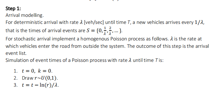
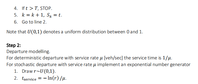
In this task, you will model a road as a queueing system. The aim is to investigate the effect of different aspects of modelling (e.g. modelling assumptions, deterministic vs. stochastic arrival and departures) on the analysis of the system and study a few performance measures of the system (e.g. average travel time). To this end, you have to develop an event-based queueing simulation (i.e. a type of model) of traffic on a single road (e.g. one street). A single road is inherently a single queue that has one state variable: the number of waiting vehicles. The events of a single queue are: arrival, service or departure, and termination. The model should keep track of each event by recording a time-sorted list of events.

We would like to see the effect of deterministic and stochastic arrivals and departures on the queueing dynamics such as number of waiting vehicles and average travel time of vehicles. For the deterministic process, you can use a uniform process while for stochastic process, you can use Poisson process.

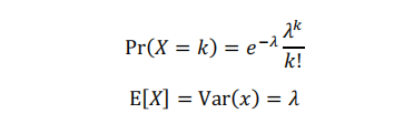
Poisson distribution: 运输系统代写

Siméon-Denis Poisson (1781–1840) was a French mathematician. The Poisson distribution is frequently used to model (or simulate) events, where events are occurring at random time points assuming events occur continuously and independently of one another. A typical usage is to model arrivals of vehicles (or customers) in a queue. The PDF, expected value, and variance of a Poisson distribution are as follows:

Step 3:

Assume the road has the length of L [m] and the free flow speed is V [m/s]. Readily, the free flow travel time is t₀ = L⁄V. In addition, assume the service rate (road capacity) is u.

Complete the event-based simulation as: Once a vehicle enters the road at time t

• the time it joins the queue ist+t0
• att+t0 increase queue by one
• ifqueue size is exactly one
  • servicetime for vehicle is tservice ~ exponential (u)
  • createdeparture event at time t + t₀ + tservice

Once a vehicle departures the road at time t  运输系统代写

• reducequeue size by one
• ifthe queue on road is still larger than zero
  • servicetime for next vehicle is tservice ~ exponential (u)
  • create departure event at time t+ tservice

Step 4:

Collect all important and useful statistics such as the arrival time and the departure time of each vehicle. With this you can construct the input-output curves and estimate the number of vehicles on the road, total travel time, and average travel time. Note that the indicators under interest are random variables. So running the simulator provides one realization of these random variables. Hence a large number of realizations must be drawn to obtain a meaningful distribution. It is not unusual to have performance measures with complex distribution that is multi-modal and asymmetric. Therefore, the mean may not always be sufficient to describe the random variable. Thoroughly compare the outputs of the model as D/M/1; M/D/1; and M/M/1 with  The arrival duration is 15 minute. Run the model until all the arrived vehicles depart.

Step 5:  运输系统代写

Assume an intersection with two approaches (each with one lane) and a two-phase traffic signal (for the sake of simplicity assume no yellow time and no all-red time). During the red phase there is no departure while during the green phase the departure follows the deterministic process with service rate u. Run Step 4, assuming D/D/1 for both roads with  The arrival duration is 15 minutes. Run the model until all the arrived vehicles depart. Consider

C=60 [sec], G=40 [sec]

C=60 [sec], G=30 [sec]

iii.

C=60 [sec], G=20 [sec]

C=90 [sec], G=60 [sec]

C=90 [sec], G=45 [sec]

C=90 [sec], G=30 [sec].

Task 3 (35%)

Public Transport Data Analysis: Analyzing Bus Trips in Sydney

Required Material:

A Spreadsheet Software (Excel)

A geographical data visualization software (e.g. QGIS)

A programming language suitable for working with big datasets (Python, R, or MATLAB)

Data files: Bus occupancy data of Sydney available at https://opendata.transport.nsw.gov.au/ The required data has been uploaded to Canvas

 Introduction: 运输系统代写

In this task, you will investigate the delay of bus stops on a number of popular routes and analyze the data from a traffic engineering point of view. You will visualize bus routes using the GPS locations provided in the datasets, perform data analysis on the timetable (expected) and actual arrival time of buses across three weeks in 2016 and 2017. The aim is to identify the hot spots of public transport including routes and stops, and to make professional suggestions to improve the operation of the on-road public transport system.

Data description:

The data contains the qualitative occupancy, GPS location, planned and actual arrival of every bus on every route of the Sydney road network over three weeks. You are encouraged to carefully read the data specifications provided by TfNSW (uploaded to Canvas). You should download the CSV file of a single day in order to understand and visualise it, as well as the whole three week dataset (which is large enough that you cannot open it in Excel). The analysis should be done on the whole dataset.

Step 1: 运输系统代写

Randomly select four high frequency routes that go through the Ultimo and Surry Hills suburbs. Each route should have at least 15 stops. Use the one-day dataset to do this task, and then visualize the data on a geographic map of Sydney. You can use QGIS to this aim, and a short introduction to this task will be given to you in class.

Step 2:

Write a program to calculate the hourly bus delays at each stop of each route during weekdays for the three weeks of data. This program should be written in a language that can handle large datasets, such as Pandas library in Python, R, or MATLAB. You should find a way to deal with missing data in the actual arrival times column.

Step 3:

Identify the stops that share multiple routes (if any). Calculate (i) average and total hourly route delay (ii) average and total hourly delay at each bus stop throughout the study period (weekdays of three weeks of data).

Step 4:

Plot the output data obtained from Step 3 in a creative and informative way. Identify the routes and stops with the largest vehicle delays and analyse the potential reasons why you observe those hotspots.

Step 5: 运输系统代写

Plot the time-space diagram of the bus movements of each route for three different days, the outbound direction, and identify the bus bunching phenomena. Here, space dimension is referring to the distance from the origin point of the bus. Is there any relationship between findings of Steps 4 and 5?

Hint: plot the trajectory of every bus service (identified by a unique trip code) with a distinguished colour. You can use figures with multiple sub-figures, wherein each subfigure demonstrates the time-space diagram of a certain route, the outbound direction, in a certain day. You can use the latitude and longitude data to measure the vehicle’s distance from its origin point for each bus trip. For instance, Haversine distance can be used to this aim1.

Step 6: (optional with bonus)

Repeat Steps 2, 3, and 4, but this time provide a rough estimation of passenger delay for each route and every stop.

Hint: you can use the Opal recorded Status, Capacity buckets, seated and standing capacity data columns to this aim.

Step 7:

Make some recommendations on how to improve the performance of the public transport network based on the results of the previous steps. You can use logics and knowledge you have gained during this course.

 

更多代写：java代写 留学生代考 留学代写 文章代写  outline代写 毕业设计代写

合作平台：天才代写 幽灵代写  写手招聘  paper代写