博客

EC220

Introduction to Econometrics

代考Econometrics The following week you receive additional data that includes a range of demographic and socio-economic variables for each constituency.

Instructions to candidates

This paper contains TWO sections. Section A contains ONE question related to Michaelmas Term and Section B contains THREE questions related to Lent Term. Answer ALL questions.

Section A carries 1/3 of the overall summer examination mark.

Section B carries 2/3 of the overall summer examination mark.

Allocate your time accordingly.

Time Allowed Reading Time:  15 minutes

Writing Time: 3 hours

You are supplied with:

Murdoch & Barnes Statistical Tables (4th ed.)

Table A5 Durbin-Watson d-statistic

You may also use:  No additional materials

Calculators: Calculators are allowed in this examination

SECTION A  代考Econometrics

Answer all questions. This section carries 1/3 of the overall mark.

1.(33 marks) Cardiovascular disease is the number-one cause of death in sub-Saharan Africa in adults over the age of 30. You have been hired by the government of Namibia to evaluate a (hypothetical) new hypertension testing regime that has been rolled out to ap-proximately 30% of administrative constituencies across the country. Free follow-up treat-ment is available to anyone who tests positive for high blood pressure; however, historically very few individuals have been screened.

(a) (5 marks) In the early stages of your analysis, the government sends you data from a cross section of 121 constituencies in 2015. The data contains information on whether the hospitals and health service points in a constituency are using the new protocols and the share of individuals being screened. Suppose you run the regression

Sharescreened_i = ε + β NewProtocols_i+ ε_i;

where ShareScreenedi is the share of individuals over the age of 30 in constituency_i who are screened, and NewProtocolsi is an indicator for whether the local health centres have adopted the new protocols. (i) What is the precise interpretation of the parameter estimates in this regression? (ii) Would you expect  to capture the causal effect of the new protocols? Explain your answer.  代考Econometrics

(b) (5 marks) The following week you receive additional data that includes a range of demographic and socio-economic variables for each constituency. What would you expect to happen to the coeffificient on NewProtocolsi if you included a control for av-erage income? Explain your reasoning and state clearly any assumptions you make.

(c) (8 marks) The next week you receive better data. Data on screening rates and all of the demographic and socio-economic characteristics for each constituency in 2010.

None of the health facilities in the country were using the new protocols in 2010, while(as noted above) approximately 30% were using them in 2013. Explain how you could use a difference-in-difference estimator to assess the effect of the new protocols.

(d) (6 marks) What is the key assumption for the difference-in-differences estimator to provide an unbiased estimate of the effect of the new protocols? Describe what other information you would like to use and what analysis you would like to do in order to check if this assumption is satisfified. If patients were aware of the new protocols and may have moved in response, how would this affect the validity of your identifying as-sumptions?

(e) (9 marks) In 2014, the government offers a small grant to constituencies that adopt the new protocols. Because of limited funds, the grants were allocated by lottery to half of those constituencies that had not adopted before 2014. In 2017, the new protocols have been adopted by 75% of those constituencies that were offered the grant and 25% of those that were not. Explain how you could use this information to assess the impact of adopting the new protocols. Carefully discuss the assumptions necessary for this approach to provide a consistent causal estimate and describe precisely for whom this estimate is valid.

SECTION B  代考Econometrics

Answer all questions. This section carries 2/3 of the overall mark.

2.(22 marks) Consider the multiple regression model

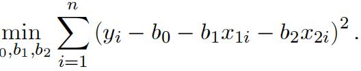
Let ( ) be the OLS estimator which minimizes the residual sum of squares

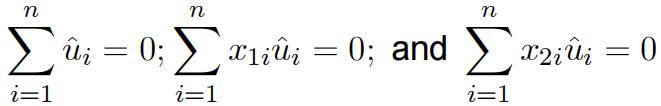
(a) (5 marks) Show that you can write the fifirst-order conditions as

(2.1)

where  is the OLS residual:

(b) In this part we want to derive the expression for (known as the regression anatomy formula): (2.2)

where are the residuals from regressing x1i on an intercept and x2i : You are told that the residuals, for the same reason as in (a), satisfy the conditions:

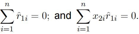
(2.3)

i.(2 marks) Let be the OLS fifitted values of the regression of x1i on an intercept and x2i , show n

(2.4)

ii.(5 marks) Using the fact that

show

(2.5)

show that can be rewritten as

show that you can obtain the expression for given in (2.2).

Let us impose the following assumptions.

MLR.1 The population model is y = β 0 + β 1×1 + β 2×2 + u.

MLR.2 We have a random sample of size n, f(yi ; x1i ; x2i) : i = 1; : : : ; ng, following the population model in MLR.1.

MLR.3 None of regressor is constant, and there are no exact linear relationships among them.

MLR.4 The error term u satisfifies E(u|x1; x2) = 0 for any value of (x1; x2)

(c) (2 marks) Explain why MLR.3 is required.

(d) (4 marks) Show that given in (2.2) is an unbiased estimator of β1 . The results (2.3), (2.4), and (2.5) may help.

(e) (4 marks) Derive the variance V ar(|X) under MLR.1-MLR.4.

3.(22 marks)

(a) (11 marks) Consider the following table of OLS regressions explaining the salary of CEO’s with the help of fifirm specifific and CEO specifific variables.

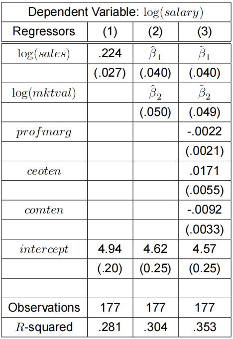
The fifirm specifific variables considered are: sales denoting fifirm sales, mktval its mar-ket value, and profmarg the profifit of the fifirm as a percentage of sales. The CEO specifific variables are: ceoten denoting the amount of years the individual has beenCEO with the current company, and comten denoting the CEO’s total years with the company. The standard errors are reported in parentheses.

i.(4 marks) Should we expect the estimate in column (2) be larger or smaller than the estimate :224 in column (1)? Explain your answer clearly.

ii.(4 marks) Test the null hypothesis H0 : β comten = 0 against H1 : β comten < 0.

Indicate how you can obtain the p-value of this test.

iii. (3 marks) Based on the above output, implement a test for the joint hypothesis H0 : β profmarg = β ceoten = β comten = 0 at 5% signifificance level. Interpret your result.

(b) (11 marks) Let us consider a simple static model to explain a city’s murder rate (mrtdrte) in terms of the murder conviction rate (convrte); local unemployment rate(unem); and the fraction of the population consisting of men between ages of 18 and 25 (yngmle)mrdrtet = β 0 + β 1 concrtet + β 2unemt + β 3yngmlet + ut ; t = 1; :::; T:

Let us assume E (u_t|s_t, s_t—1, …) = 0 where s_t = (concvte_t, unem_t, yngm1e_t) . You sus- pect that the errors exhibit autocorrelation.

i.(3marks) Give two examples of covariance stationary error processes that dis- play  Provide a clear discussion revealing the distinctive nature of their dependence patterns.

ii.(4 marks) Discuss for the given model the consequences for the ordinary least squares estimator  (unbiasedness, efficiency and consistency) in the presence of autocorrelation. Support your answers with suitable

iii.(4 marks) Answer either or the following twoquestions

EITHER

Discuss how you would detect the presence of autocorrelation in the errors in this model. Clearly indicate the null and alternative hypothesis, the test statistic, re-jection rule, and indicate the assumptions underlying your test.

OR

The above model is not very interesting when we have time series data as it ignores any dynamics in this relationship. Discuss a modifification of the above model that you might want to propose and the ideas behind your suggestion(s).Comment on the effect this might have on the evidence of autocorrelation.

4. (22 marks)  代考Econometrics

(a) Consider a model to estimate the effects of smoking on annual income

(4.1)

where cigs is the average number of cigarettes smoked per day and educ is the years of schooling (without loss of generality we are not considering age; age2 and ethnicity). To reflflect the fact that cigarette consumption may be jointly determined with income, we postulate the following demand for cigarettes equation:

cigs = 1 + 2 log (income) + 3 educ + 4 log (cigpric) + 5 restaurn + u;(4.2)

where cigpric is the price of a pack of cigarettes (in cents), and restaurn is a binary variable equal to unity if the person lives in a state with restaurant smoking restrictions.

The endogenous variables in this model are log(income) and cigs; and the exogenous variables are educ; log(cigpric) and restaurn:  代考Econometrics

You collect a random sample of observations and may assume the zero mean er-rors (ε; u) are homoskedastic and

i.(2 marks) The above equations provide the structural equations whose parame-ters we are interested in estimating. Interpret the parameters β2 and 2 :

ii.(5 marks) What does it mean to say that in equation (4.1), we treat educ as being exogenous and cigs as being endogenous? Provide a proof of the endogeneity of cigs; clearly indicating what assumptions you are making use of. In your answer you are expected to derive the reduced form for cigs:

iii. (4 marks) In view of the endogeneity, prove that the OLS estimator of β2 will be inconsistent. In your answer, you may set β3 = 0 for simplicity. Explain why the inconsistency of your OLS estimator is not surprising.

iv.(6 marks) Providing the intuition behind the approach, indicate how/whether you can obtain consistent estimates of β2 and 2 : What assumptions are needed for

this result? In your answer you should indicate whether (and under what con-ditions) (4.1) and (4.2) are (i) under-identifified, (ii) exact-identifified, or (iii) over-identifified, and explain this terminology.

(b) (5 marks)

Answer either of the following two questions.

EITHER

You want to make the above model more realistic by adding an equation representing the supply for cigarettes. In this augmented model, log(cigpric) will be endogenous as well. Discuss how supply shifters (such as cost of processing tobacco and weather)can be used in our quest to obtain consistent estimates of 2 in part (a).

OR

You are interested in explaining the probability of an individual smoking. Let us ig-nore the possible endogeneity between cigarette consumption and income. Given the above data, you generate a dummy variable smoke which indicates whether cigs > 0(smoke = 1) or not (smoke = 0):

Discuss the drawbacks and advantages of using the Linear Probability Model when trying to explain the binary decision indicating whether you smoke or not. In your answer clearly indicate what the Linear Probability Model is. Brieflfly indicate what alternative you want to propose to remedy the main drawback.]

 

更多代写：加拿大网课代修价格  gre替考  经济学代考价格  金融Essay代写范文  教育学论文写作  Date an alysis 代写

合作平台：essay代写 论文代写 写手招聘 英国留学生代写