EC220
Introduction to Econometrics
代写计量经济学作业 If these businesses cannot borrow freely they may have to rely on the private resources of the owners to fifinance their business activities.
Instructions to candidates 代写计量经济学作业
This paper contains TWO sections. Section A contains ONE question related to Michaelmas Term and Section B contains THREE questions related to Lent Term. Answer all.
Section A carries 1/3 of the overall summer examination mark.
Section B carries 2/3 of the overall summer examination mark.
Allocate your time accordingly
Time Allowed Reading Time: 15 minutes
Writing Time: 3 hours
You are supplied with: Murdoch & Barnes Statistical Tables
Table A5 Durbin-Watson d-statistic
You may also use: No additional material
Calculators: Calculators are allowed in this examination
Section A 代写计量经济学作业
(Answer all questions. This section carries 1/3 of the overall mark)
Question 1 [33.33 marks]
The lack of access to suffificient credit may be an important impediment for the growth of small busi-nesses. If these businesses cannot borrow freely they may have to rely on the private resources of the owners to fifinance their business activities. Economists therefore have investigated whether the private wealth or collateral of owners of small businesses matters for business growth.
The following regressions are for 9,125 individuals who started being self-employed in 2012. The empirical strategy of the study is to compare various business outcomes (assets, sales, and number of employees) for homeowners and renters in 2017. The regressions also interact homeownership status with house price appreciation in the region of residence. Homeowners, who see their houses become more valuable, may often have access to mortgage fifinancing which could be used to invest in their business. House price growth is coded so that growth of 5% would be 0.05.
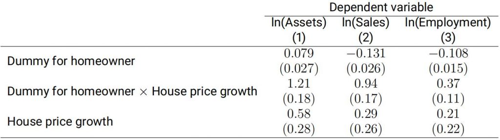
Standard errors are displayed in parentheses. All regressions also contain a constant term.
(a)Explain why a simple regression of business outcomes on the wealth of the owner may not answer the question economists are interested in.[5.33 marks]
(b)Explain how the use of house price growth may circumvent the problem you described in part(a).[7 marks]
(c)Explain verbally what the coeffificient of 0.079 on the dummy for homeowners in column (1) means.[3 marks]
(d)If house price growth is 10 percentage points higher, how much higher are the sales of renters in the sample on average? Explain whether this effect is statistically different from zero.[5 marks]
(e)What do you conclude from the results in the table about the effect of owner collateral on busi-ness outcomes?[6 marks]
(f)Suppose you also have data for assets, sales, and employment in these businesses in 2012.Suppose you were to run analogous regressions with these dependent variables to the regres-sions in the table above. Explain how the new regressions would help you interpret the results above.[7 marks]

Section B 代写计量经济学作业
(Answer all questions. This section carries 2/3 of the overall mark)
Question 2 [22.33 marks]
Consider the bivariate regression model without intercept
yi = βxi + ui , (2.1)
for i = 1, . . . , n. We impose the following assumptions.
SLR.1 The population model is y = βx + u.
SLR.2 We have a random sample of size n, {(yi , xi) : i = 1, . . . , n}, following the population model in SLR.1.
SLR.3 The sample outcomes on{xi : i = 1, . . . , n} are not all the same value.
SLR.4 The error term u satisfifies E(u|x) = 0 for any value of x.
SLR.5 The error term u satisfifies V ar(u|x) = σ 2 for any value of x (homoskedasticity).
(a)Consider the OLS estimator
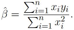
Under SLR.1-5, derive the (conditional) variance V ar(βˆ|X), where X = (x1, . . . , xn).[5 marks]
(b)Suppose additional data become available, and we have a random sample of size 2n, {(yi , xi) : i = 1, . . . , 2n}, which satisfy SLR.2-3 above. Now we can implement the OLS estimator
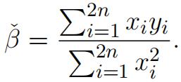
Compare βˆ and βˇ in terms of effificiency and consistency.[4.33 marks]
(c)Now, consider the following estimator
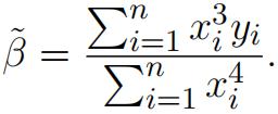
Show that β˜ is unbiased under SLR.1-5.[4 marks]
(d)Explain how to test the homoskedasticity assumption in SLR.5.[5 marks]
(e)Suppose SLR.5 is violated, and instead it is known that
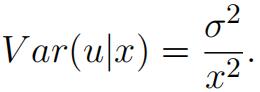
In this case, show that β˜ in (c) is the generalized least square (GLS) estimator.[4 marks]
Question 3 [22.33 marks]
(a)Are rent rates inflfluenced by the student population in a college town? Let rent be the averagemonthly rent paid on rental units in a college town in the United States. Let pop denote the total city population, avginc the average city income, and pctstu the student population as a percentage of the total population. One model to test for a relationship is
log(rent) = β0 + β1 log(pop) + β2 log(avginc) + β3pctstu + u.
The equation estimated using data from 64 college towns is
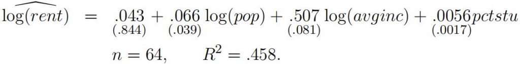
(i)Explain brieflfly how to interpret the estimate for β1. If we replace pop in the above regression with popthousand = pop/1000 (measured in thousands), what will happen to the OLS estimates for β0 and β1?[4 marks]
(ii) State the null hypothesis that size of the student body relative to the population has no ceteris paribus effect on monthly rents. State the alternative that there is an effect. Then explain how to compute the p-value for this test. Draw a sketch to illustrate.[3.33 marks]
(iii) Suppose you want to test the joint hypothesis H0 : β1 = β2 = 0. In addition to the above regression output, explain what kind of output do you need. Then explain how to implement the test for H0.[3 marks] 代写计量经济学作业
(b)In this part we consider the expectations augmented Phillips curve (see also Mankiw, 1994):
inflflt − inflfle t= β1 (unem0 − µ0) + et ,
where µ0 is the natural rate of unemployment (assumed to be constant over time) and inflflet is the expected rate of inflflation formed in t − 1.This model suggests that there is a tradeoff be-tween unanticipated inflflation (inflflt -inflfle t ) and cyclical unemployment (difference between actual unemployment and the natural rate of unemployment).
We assume that et (also called supply shock) is an iid random variable with zero mean. You are told that expectations are formed using the following adaptive expectation model:
inflflet − inflfle t-1 = λ(inflt-1 – inf et-1) .
Given this information, it can be shown (you are not asked to do this) that the model can be written as:
∆inflflt = γ0 + γ1unemt + γ2unemt-1 + vt , (3.1)
where ∆inflflt =inflflt−inflflt-1, γ0 = −β1λµ0, γ1 = β1, γ2 = −(1 − λ)β1, and
vt = et − (1 − λ) et-1. (3.2)
(i) What name do we give the process vt in (3.2)? Is this process covariance stationary and weakly dependent? Brieflfly discuss.[3 marks]
(ii) Discuss what (minimal) assumptions you need to make about et (the supply shock) to guar-antee the consistency of the OLS estimator for (γ0, γ1, γ2) in (3.1). (You are not expected to prove its consistency.)
Indicate how you can use the consistency of the OLS estimator for (γ0, γ1, γ2) to obtain a consistent estimator for the long run effect of unemployment on the change in inflflation. Prove your claim.[5 marks]
(iii) Let the assumptions for consistency of of the OLS estimator for (γ0, γ1, γ2) in (3.1) be satisfified. How can you obtain valid standard errors for the long run effect of unemployment on the change in inflflation?
Question 4 [22 marks] 代写计量经济学作业
(a)An economist is interested in estimating the production function for widgets which is postulated to follow a Cobb-Douglas specifification:
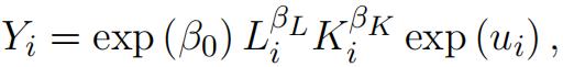
where Yi is a measure of output for fifirm i, Li is labor, Ki is capital stock and ui is an un-observed term that captures technological or managerial effificiency and other external factors(e.g., weather). The parameters to be estimated are (β0, βL, βK). Taking logs,
ln Yi = β0 + βL ln Li + βK ln Ki + ui .
(i) Assume that you have a cross-section of independent fifirms and that more productive fifirms hire less workers (labor). Explain why OLS would not provide consistent estimates for (β0, βL, βK). Would it over- or underestimate βL on average? Clearly explain your answer.[5 marks]
Instead of applying OLS, the economist decides to use the average wage paid by fifirm i, Wi , as an instrument for the (log) quantity of labor employed by that fifirm, ln Li .
(ii) Describe in detail how you would estimate the parameters of the production function us-ing Two Stage Least Squares (2SLS). What restrictions would be necessary for this re-searcher to successfully use this instrumental variable in the estimation of the parameters(β0, βL, βK) and what would you need to assume about capital stock?[6 marks]
(iii) If average wages per fifirm do not vary much by fifirm (potentially because of unionization or high mobility of the labor force), how would this affect the properties of the estimation procedure suggested in (ii)? Explain your answer.[4 marks]
(b)In this part, we are interested in analysing whether workplace smoking bans affects the inci-dence of smoking. Using data on 10,000 US indoor workers from 1991 to 1993 taken from “Do Workplace Smoking Bans Reduce Smoking”, by Evans et al. (American Economic Review, 1999),the following probit regression was estimated.
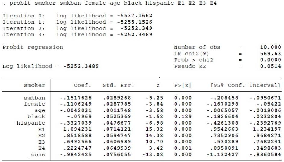
The dependent variable, smoker, is a dummy variable indicating whether a worker smokes (1=yes,0=no) and the explanatory variables are smkban, a dummy variable indicating whether there is a ban on smoking in the workplace (1=yes, 0=no), the worker’s age (in years), gender (male/female),ethnicity (black/hispanic/white) and level of education (E1=highschool dropout, E2=highschool graduate, E3=some college, E4=college graduate, E5 Master degree or above).
(i) Test whether these results show that smoking in the work place has a signifificant effect on the incidence of smoking.[3 marks]
(ii) Explain how you can estimate the effect of the smoking ban on the probability of smoking for a 50-year old white, college graduated man. You are not expected to use your calculator,clarity of the computations required is enough.
Hint: You may recall that for the Probit model, we will specify
P r(smoker = 1|x) = Φ(β0 + β1smkban + β2female + …β8E3 + β9E4)
where Φ is the standard normal CDF (cumulative distribution function).[4 marks]
更多代写:online quiz代考价格 sat考试作弊 Economics经济学商科代写 essay代写美国 literature review代写推荐 英语论文
合作平台:essay代写 论文代写 写手招聘 英国留学生代写