Machine Learning
代做机器学习作业 A single pdf report should be submitted on QMplus along with the completed Notebooks for both this and the Neural Networks notebook (lab 6).
0. Introduction 代做机器学习作业
The aim of this lab is to get familiar with classification problems and logistic regression.We will be using some code extracts that were implemented last week and build a logistic regression model.
1.Thislab is part of Assignment 1 part 2.
2.A report answering the **questions in red** should be submitted on QMplus along with the completed Notebooks.
3.A single pdf report should be submitted on QMplus along with the completed Notebooks for both this and the Neural Networks notebook (lab 6).
4.The deadline for both is Friday, 18 November11:59pm 代做机器学习作业
5.Thereport should be a separate file in pdf format (so NOT doc, docx, notebook ), well identified with your name, student number, assignment number (for instance, Assignment 1), module code.
Makesure that any figures or code you comment on, are included in the report .
Noother means of submission other than the appropriate QM+ link is acceptable at any time (so NO email attachments, )
PLAGIARISMis an irreversible non-negotiable failure in the course (if in doubt of what constitutes plagiarism, ask!).
For this lab, we will be using the iris dataset.
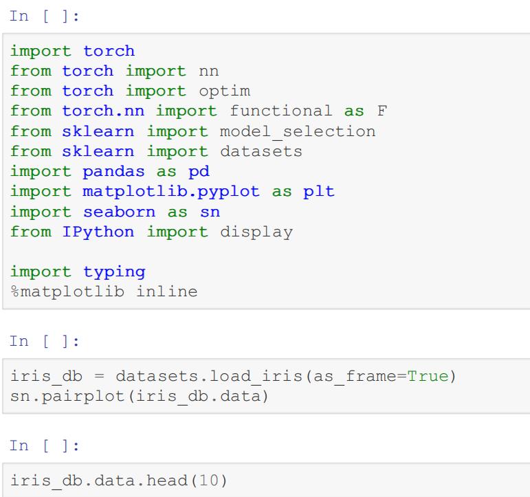
We will split the data into train and test sets. For consistency and to allow for meaningful comparison the same splits are maintained in the remainder of the lab.
In [ ]:
X_train, X_test, y_train, y_test = model_selection.train_test_split(
iris_db.data,
iris_db.target,
test_size=0.2,
random_state=42
)
x_train = torch.from_numpy(X_train.values).float()
x_test = torch.from_numpy(X_test.values).float()
y_train = torch.from_numpy(y_train.values).int()
y_train = y_train.reshape(-1, 1)
**Q1.** We again notice that the attributes are on different scales. Use the normalisation method from last lab, to standardize the scales of each attribute on both sets. Plot the normalized and raw training sets; what do you observe? [2 marks] 代做机器学习作业
In [ ]:
### your code here
By inspecting the dataset we see that it contains 4 attributes. (sepal length,sepal width,petal length,petalwidth, in centimeters). For simplicity we will focus on the first two.
In [ ]:
X = iris_db.data.iloc[:, :2]
Y = iris_db.target
marker_list = [‘+’, ‘.’, ‘x’]
fig = plt.figure(figsize=(7, 7))
ax = fig.add_subplot(111)
ax.set_aspect(‘equal’)
for l in [0, 1, 2]: ax.scatter(
X.loc[Y == l].iloc[:, 0],
X.loc[Y == l].iloc[:, 1], marker=marker_list[l],
s=70,
color=’black’,
label='{:d} ({:s})’.format(l, iris_db.target_names[l])
)
ax.legend(fontsize=12)
ax.set_xlabel(iris_db.feature_names[0], fontsize=14)
ax.set_ylabel(iris_db.feature_names[1], fontsize=14)
ax.grid(alpha=0.3)
ax.set_xlim(X.iloc[:, 0].min() – 0.5, X.iloc[:, 0].max() + 0.5)
ax.set_ylim(X.iloc[:, 1].min() – 0.5, X.iloc[:, 1].max() + 0.5)
plt.show()
Is the data linearly separable?
As there are multiple classes, for now we will focus on class 0 (setosa). As such, we modify the tensors, so that each label is 1 if the class is setosa and 0 if otherwise.
In [ ]:
train_set_1 = x_train[:, :2]
test_set_1 = x_test[:, :2]
# add a feature for bias
train_set_1 = torch.cat([train_set_1, torch.ones(train_set_1.shape[0], 1)], dim=1)
test_set_1 = torch.cat([test_set_1, torch.ones(test_set_1.shape[0], 1)], dim=1)
setosa_train = (y_train == 0).int()
setosa_test = (y_test == 0).int()

1. Sigmoid function 代做机器学习作业
With logistic regression the values we want to predict are now discrete classes, not continuous variables. In other words, logistic regression is for classification tasks. In the binary classification problem we have classes 0 and 1, e.g. classifying email as spam or not spam based on words used in the email.
The logistic/sigmoid function given by the formula below:
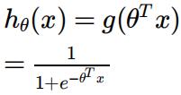
Q2. First implement the above function in def sigmoid() . [2 marks]
Q3. Then, using the implementation of LinearRegression from last week as guideline, create a custom pytorch layer for LogisticRegression [2 marks]
In [ ]:
def sigmoid(z: torch.Tensor) -> torch.Tensor:
### your code here
return z
x = torch.arange(1,2000, 1)/100.0 – 10
y = sigmoid(x)
fig, ax1 = plt.subplots()
ax1.plot(x, y)
# set label of horizontal axis
ax1.set_xlabel(‘x’)
# set label of vertical axis
ax1.set_ylabel(‘sigmoid(x)’)
plt.show()
In [ ]:
class LogisticRegression(nn.Module):
def __init__(self, num_features):
super().__init__()
self.weight = nn.Parameter(torch.zeros(1, num_features), requires_grad=False) 代做机器学习作业
def
forward(self, x):
y = 0
### your code here
return y
The cost function we will use for logistic regression is the Cross Entropy Loss , which is given by the form:
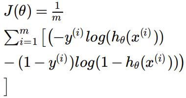
Which when taking partial derivatives and putting these into the gradient descent update equation gives
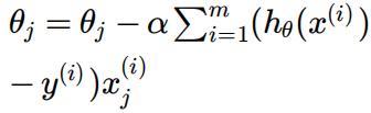
Q4. Implement the cost in and update the from last week to update using the partial derivative above. [4 marks]
In [ ]:
def bce(y_true: torch.Tensor, y_pred: torch.Tensor) -> torch.Tensor:
### your code here
return
def gradient_descent_step(model: nn.Module, X: torch.Tensor, y: torch.Tensor, lr: float)
-> None:
weight = model.weight
N = X.shape[0]
### your code here
###
model.weight = nn.Parameter(weight, requires_grad=False)
In [ ]:
def train(model, x, y, alpha):
cost_lst = list()
for it in range(1000):
prediction = model(x)
cost = bce(y, prediction)
cost_lst.append(cost)
gradient_descent_step(model, x, y, alpha)
display.clear_output(wait=True)
plt.plot(list(range(it+1)), cost_lst) 代做机器学习作业
plt.show()
print (model.weight)
print (‘Minimum cost: {}’.format(min(cost_lst)))
model = LogisticRegression(train_set_1.shape[1])
alpha = 1 # select an appropriate lr
train(model, train_set_1, setosa_train, alpha)
**Q5.** Draw the decision boundary on the test set using the learned parameters. Is this decision boundary separating the classes? Does this match our expectations? [2 marks]
In [ ]:
### your code here
2. Multiclass 代做机器学习作业
So far, we have focused on a binary classification (is this iris setosa or not), however in this section we will address the problem as a multiclass classification. We will be using a 1 vs. all approach (refer to the lecture notes for details). We will also be using all 4 attributes for the classification.
Firstly, we need to process y_train, y_test so that each label is a vector rather than an integer.
In [ ]:
y_train = F.one_hot(y_train.reshape(-1).long(), num_classes=3)
y_test = F.one_hot(y_test.reshape(-1).long(), num_classes=3)
print(y_test.shape)
In this section we will use the built in pytorch methods.
In [ ]:
alpha = 0.1
setosa_model = nn.Sequential(nn.Linear(x_train.shape[1], 1, bias=False), nn.Sigmoid())
setosa_labels = y_train[:, 0].reshape(-1, 1).float()
setosa_testy = y_test[:, 0].reshape(-1, 1).float()
optimiser = optim.SGD(setosa_model.parameters(), alpha)
def train(model, x, y, test_x, test_y, optimiser, alpha):
train_lst = list()
test_lst = list()
for i in range(1000):
model.train()
optimiser.zero_grad()
pred = model(x)
cost = F.binary_cross_entropy(pred, y, reduction=’mean’)
cost.backward()
train_lst.append(cost.item()) 代做机器学习作业
optimiser.step()
model.eval()
with torch.no_grad():
test_pred = model(test_x)
test_cost = F.binary_cross_entropy(test_pred, test_y, reduction=’mean’)
test_lst.append(test_cost)
fig, axs = plt.subplots(2)
axs[0].plot(list(range(i+1)), train_lst)
axs[1].plot(list(range(i+1)), test_lst) plt.show()
print(‘Minimum train cost: {}’.format(min(train_lst)))
print(‘Minimum test cost: {}’.format(min(test_lst)))
In [ ]:
train(setosa_model, x_train, setosa_labels, x_test, setosa_testy, optimiser, alpha)
How does the cost of the 4 attribute model compare to the previous one?
Q6 Now train classifiers for the other two classes.[1 mark]
In [ ]:
### your code here
**Q6.** Using the 3 classifiers, predict the classes of the samples in the test set and show the predictions in a table. Do you observe anything interesting? [4 marks]
In [ ]:
### your code here
**Q7.** Calculate the accuracy of the classifier on the test set, by comparing the predicted values against the ground truth. Use a softmax for the classifier outputs. [1 mark]
In [ ]:
3. The XOR problem 代做机器学习作业
**Q8.** Looking at the datapoints below, can we draw a decision boundary using Logistic Regression? Why?What are the specific issues or logistic regression with regards to XOR? [2 marks]
In [ ]:
x1 = [0, 0, 1, 1]
x2 = [0, 1, 0, 1]
y = [0, 1, 1, 0]
c_map = [‘r’, ‘b’, ‘b’, ‘r’]
plt.scatter(x1, x2, c=c_map)
plt.xlabel(‘x1’)
plt.ylabel(‘x2’)
plt.show()
更多代写:工科作业代写 雅思作弊 高中网课代看 bio essay代写 Accounting论文代写 ECO经济学代考
合作平台:essay代写 论文代写 写手招聘 英国留学生代写