Assignment-Econ 659
Economics经济学商科代写 It is permitted to consult with other students regarding the assignment questions, however the final work submitted must be your own.
Instructions:
Penalty for late assignments = 5% per day (i.e. 5% of marks).
It is permitted to consult with other students regarding the assignment questions, however the final work submitted must be your own. Students who submit identical (or nearly identical) assignments will receive a grade of zero.
You may used Matlab, Octave, R or Python for computations and to plot graphs. Note that Octave is an open access software that is compatible with Matlab. I provide some code in Matlab (which will run in Octave) which you can use to create code in R or Python if you pre- fer. The University of Waterloo has a site license for Matlab and students are eligible to down- load and install Matlab on their personally-owned computers or used Matlab Online in a web browser. Information is available here: https://uwaterloo.atlassian.net/wiki/spaces/ STKB/pages/284525621/Download+or+use+MATLAB+online. Octave may be downloaded from this site: https://www.gnu.org/software/octave/index.
Please insert your figures as images into your assignment or submit as separate pdf files.Make sure you clearly label your graphs. Also submit the code to create your graphs.
Questions economics经济学商科代写
1.(14 marks) Note: At the end of this assignment there is an overview of solving ordinary differential equations.
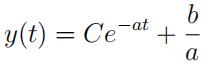
(a)(2 marks) Show that the general solution to the homogeneous form of Equation
(a)is given by yh(t) = Ce—at where C is an arbitrary constant of integration.
y˙ + ay = b (1)
(b)(2 marks) For the following di↵erential equations, state whether each equation is linear or non-linear, the order of the equation, and whether the equation is autonomous or non-autonomous. Find the solution for each equation given the initial conditions. Detail the steps needed to find the solution. Determine the limit of y for t →∞.
i.2y˙ +1y = 12 with the initial condition that t0 = 0 and y(t0) = 10.
ii.y˙— 3t—2y = t—2 with the initial condition t0 = 1 and y(t0) = 100.
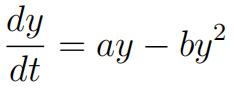
(c)(5marks) Consider a fishery in which there is no harvesting of Suppose the growth rate in a population of fish is related to the stock of fish according to . economics经济学商科代写
 (2)
(2)
where y represents the stock of fish (in tonnes) and a and b are constants. Suppose a = 4 and b = 0.1.
i.State whether this equation is linear or non-linear, the order of the equation, and whether it is autonomous or non-autonomous. Plot a graph showing dy/dt versus yfor 0 y for 0 ≤ y ≤ 45.
ii.Now suppose that a commercial fishing operation is started and the harvest rate h in this fishery is a constant h = Add a line showing this constant harvest rate in the graph created in part (i). What is/are the potential steady state(s) of the fish stock (i.e. when dy/dt = 0) given this constant harvest rate.Are these steady state stable or unstable? In other words if the fish stock is perturbed slightly above or below the steady state(s), will it tend to be pushed back towards the steady state (a stable steady state) or away from the steady state (an unstable steady state).
iii.Now suppose that the harvest rate is a function of the stock of fish according to h = ↵y, with ↵ = 0. Sketch this harvest function on your graph. What is/are the steady state fish stock level(s)? Is/are the steady state(s) stableor unstable? economics经济学商科代写
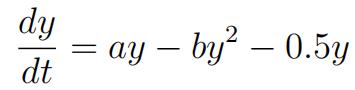
(d)(3 marks) With the harvest function h= 0.5y, the growth rate in the fish stock referred to in part 1c may be described according to:
 (3)
(3)
Specify a new variable x = f (y) with f (y) defined such that Equation (3) can be solved with linear techniques. Solve Equation (3) for the initial condition y(0) = 0.2. Show the details of your solution. Plot y as a function of time showing how y evolves to reach a steady state.
2.(6 marks)In this example you will plot the profit from buying vanilla options.
(a)Financial options can be used for speculation. Suppose you think that ZZZ com- pany will increase in value over the next 3 months. You are considering whether to buy ZZZ shares or buy call options on ZZZ shares. Suppose ZZZ’s stock price is currently 10 and a 3-month call option with a 50 strike price currently sells 2. Suppose you have 1000 to invest. Plot a graph showing the present value of profit for these two strategies versus the stock price at the exercise time.Use a discount rate of 3%. Discuss the benefits versus costs of the strategies.
(b)Financial options are also used for hedging. Suppose you own 1000 shares ofXYZ company which are currently priced at 50 per share. Suppose you anticipate the price of XYZ will decline over the next three months. You decide to hedge your position by buying 1000 put options on XYZ with an exercise price of 50 selling for 5 per option. Plot a graph showing the present value of profit of your portfolio after 3 months for the hedged and unhedged positions versus the stock price. Use a discount rate of 3%. Discuss the benefits versus costs of hedging your position. economics经济学商科代写
3.(12 marks) This question analyzes a firm’s investment in an oil field which can be madeimmediately or one year hence.
(a)(3 marks) The price of oil is currently 65 per barrel. The cost of drilling the oilwell is 1,500,000. Once in operation it costs 50 per barrel to produce the oil. It is expected that the oil well will be able to produce 20,000 barrels of oil per year for many years in the future. For the purposes of this analysis, assume constant production can be maintained forever. (Also assume that revenues are received and costs are incurred instantaneously at the beginning of each year.)
The price of oil next year is uncertain. There is a 50% chance that the price will rise to 86.5 next year and a 50% chance that the price will fall to 50. In subsequent years assume the price of oil will stay constant forever. The firm can shut down production if it is optimal to do so. The risk free interest rate is 10%. Determine the value of this investment opportunity using the dynamic programming approach. Show the steps of your calculation in detail. What is the optimal action for the firm if it owns the land already? Suppose it will cost 2.5 million to acquire the land. Would you recommend making this investment? Explain.
(b)(3 marks) Repeat the analysis of part (a) using contingent claims analysis –e.
by creating a hedging portfolio that includes the project and a short sale of oil contracts. Demonstrate that you will get the same result as in part (a). Make any necessary assumption regarding a payment required for the short sale. Explain your assumption.
(b)(3marks) On LEARN you will find a Matlab m-file called“as1 Q3 ec659f2022.m”. This file sets up the problem and calculates solutions for a vector of possible initial prices, using a standard approach dynamic program- ming approach and using a contingent claims approach. Use Matlab to plot a graph showing the value of immediate investment versus price and the value of delaying investment versus price. Make sure you label your graph clearly. What are the approximate values of the lower and upper critical prices? Discuss the meaning of the graph in terms of the firm’s optimal actions. Explain why for some initial prices of oil it is better to delay the decision, while for others it is better to invest right away. economics经济学商科代写
(d)(3 marks)Now suppose that price in the future has become more uncertain. In the next year the price may jump up to 5 times the current level, or fall to 0.5 times the current level. Rerun your Matlab program from part (c) with this new level of uncertainty. Comment on and discuss the impact of this change on the value of the investment and the critical initial prices. Also comment on the e↵ect of this change on the required dividend payment for the short sale.
4.(6 marks) In this question you will explore some properties of Brownian motion.Let economics经济学商科代写
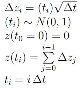
(a)Write Matlab code to simulate the path of z over Let the ending time be T = 2 and the number of timesteps be n = 400. This implies a timestep size of equals T/n = 0.005 of a year. Plot z and the variance of z over time for 10 pathsand then for 1000 paths. Compare the plots for the di↵erent number of simulations. Are they as expected for Brownian motion? Explain.
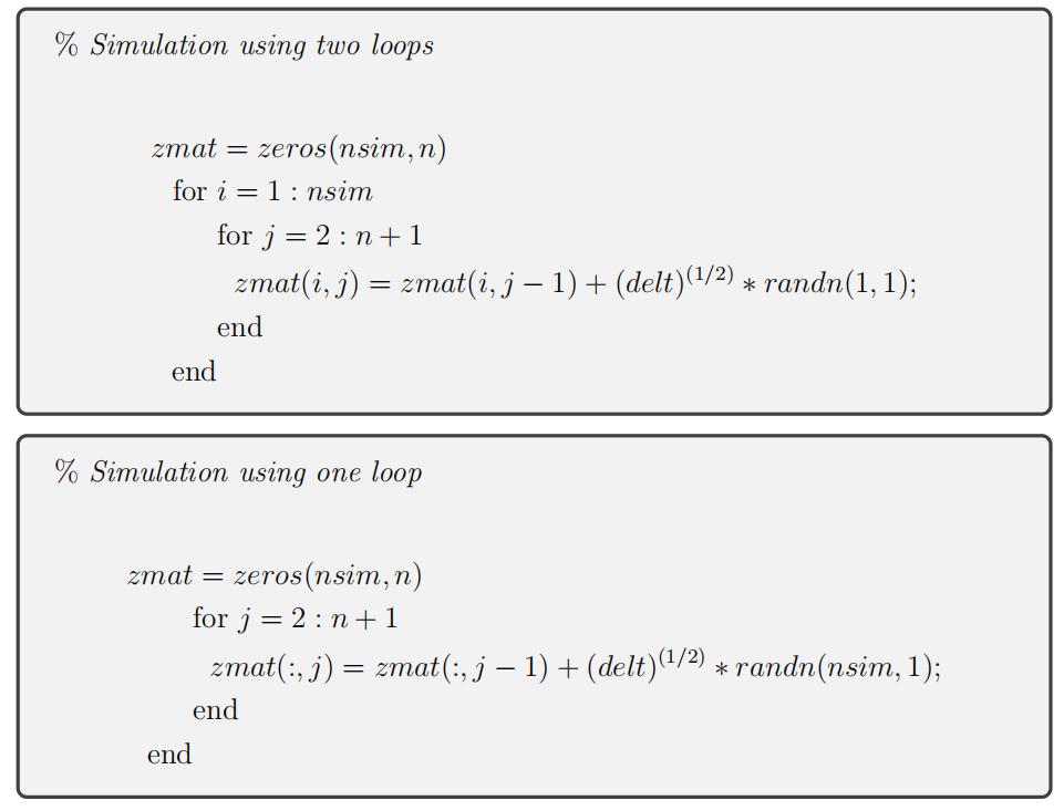
Help with Matlab coding: 1To do the simulations create an m-file in Matlab. The Matlab command ‘randn(m,n)’ generates an m-by-n matrix of pseudo-random values drawn from a standard normal distribution. Type ’help randn’ in Matlab for more information.
Three helpful commands at the beginning of your code are: clear, close all, and randn(’state’,100). The latter command means that you will get the same random number sequence whenever you run the program. Put a semicolon at the end of a line to suppress printing.
To do a single simulation construct a loop over timesteps, finding all z(j), where j is the index for the timestep. To do multiple simulations you can create a matrix
1I am unable to help with coding in R or Python, but you are welcome to use either of these. economics经济学商科代写
x mat(i,j) where i indexes the simulation number and j indexes the timestep. You can then do a double loop over i and over j to create the matrix. Alternately you can “vectorize” your code defining each column as a vector. The latter approach is more efficient in Matlab, meaning your code will run faster. (It will not make a noticeable di↵erence in this example, but in a future assignment you will notice a significant difference.)
To get you started here is some code showing the two different approaches.
These create a matrix where each row is a single realization and there are ‘nsim’ rows.
(b)b)Consider the function of z defined as follows.
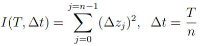
Write Matlab code to evaluate I(T, Ot)for T = 2. Use 1000 paths and compute the mean and variance of the result for n = 100, 200, 400, 800, 1600, 3200 timesteps. Provide a table of the mean and variance of I(T, Ot) for the di↵erent values of Ot. Plot a graph of the variance of I(T, Ot) versus Ot. Discuss the result and relate it to a crucial step in deriving Ito’s lemma.

5.(5 marks) Consider the generalized Wienerprocess: economics经济学商科代写
dx = 0.3dt + 0.3dz. (4)
Suppose the initial value of x is x0 = 1.
(a)Calculatethe expected value of x after 2 years.
(b)Calculatethe standard deviation of x after 2 years.
(c)Determinea 95% confidence interval for x after 2 years.
(d)Consider a European call option on this asset with an exercise price of 2 andexpiry date in 2 years. What is the probability that this option will be exercised at expiry? Show your work in detail.
(e)What is the probability that a European put option on this asset with the same maturityand exercise price will be exercised?
6.(8 marks) Consider the GBM process:
dS = 0.3Sdt + 0.3Sdz. (5)
Suppose the initial value of S is S(0) = 1.
(a)Calculatethe expected value of S after 2 years.
(b)Calculatethe standard deviation of S after 2 years.
(c)What can you say about the distribution of Y = log(S) after 2 years? What are its expected value and standarddeviation?
(d)Find a 95% confidence interval for Y after 2 years. Use your results to calculate a 95% confidence interval for S.
(e )Write Matlab code to simulate the path of Y over 2 years for 100 and 1000 paths. Convert your simulation values from Y to S. Find estimates of the standard devi- ations and means at T=2 for Y and S. Compare your answers for the 100 versus 1000paths to the exact values calculated in (a) through (c) Comment on the differences. Create graphs of the simulations of Y versus time and S versus time for the 1000 simulation case. Compare the shapes of the two graphs.
1 Brief review of ordinary differential equations economics经济学商科代写
A differential equation is a relation between an unknown function and its derivative. If the unknown function is a function of one variable only the relation is referred to as an ordinary differential equation; if it is a function of several variables (so that the equation contains partial derivatives), it is called a partial di↵erential equation. The order of a differential equation is that of the derivative of the highest order occurring in it.
A first order ordinary di↵erential equation is an equation of the form
F (t, y, y˙) = 0 (6)
where y˙ ⌘ @y/@t, or in the special case where the equation is solved for y˙:
y˙ = f (t, y) (7)
By a solution of Equation (6), we mean any function y = g(t) which satisfies Equation (6) in the domain considered.
Below is an overview of solving linear ODEs. When a di↵erential equation is nonlinear, no single solution technique will work in all cases, and only a few special cases can be solved.
1.1 Autonomous linear ODEs equations economics经济学商科代写
The general form of the linear, autonomous, first-order di↵erential equation is
y˙+ ay(t) = b (8)
where a and b are known constants. It is referred to as autonomous because a and b do not depend on t. This type of di↵erential equation can be solved by separating the problem of finding a general solution for Equation (8) into two simpler sub-problems. Let yh denote the solution to the homologous form obtained by setting b=0. Let yp denote a particular solution to the complete equation. Then the general solution can be shown to be the sum:
y = yh + yp (9)
The homogeneous form of Equation (8) is
y˙+ ay = 0 (10)
The general solution to the homogeneous form of Equation (8) is given by yh(t) = Ce—atwhere C is an arbitrary constant of integration. economics经济学商科代写
A particular solution to the complete di↵erential equation that is easy to find (if it exists) is the steady state solution where y˙ = 0. Substituting y˙ = 0 into Equation (8) gives y¯ = b where y¯ refers to the steady state solution, as long as a = 0. Substituting into Equation (9) we get the general solution to the complete autonomous, linear first order di↵erential equation.
 (11)
(11)
If an initial value for y at t = t0 is provided, we can determine the value of the constant C. Note that if a steady state solution does not exist, then a solution to Equation (8) can be found by direct integration.
1.2 Non-autonomous linear ODEs equations economics经济学商科代写
The previous approach works only when a and b are constants. A more general solution technique exists which will work for any linear, first-order di↵erential equation.
The general form of the linear, first order di↵erential equation is:
y˙ + a(t)y = b(t) (12)
where a(t)and b(t)are known continuous functions of t.
The solution technique is to multiply both sides of the di↵erential equation by a term called the integrating factor. This transfoIrnmtsetgheradit↵inergefntaiacl etqouartion so that it can be solved by direct integration. The integrating factor is given below:
Integrating factor = e(A(t)), where A(t) = s a(t)dt
Multiply Equation (12) by the integratfintg factor:
eA(t)[y˙+ a(t)y] = eA(t)b(t) (13)
You can show that the left hand side of Equation (13) is equal to:
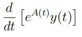 (14)
(14)
Therefore Equation (13) can also be written as:
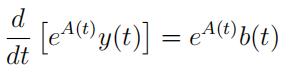 (15)
(15)
This form of the equation can be solved by direct integration which, after rearranging, gives:
y(t) = e—A(y) [∫ eA(t)b(t)dt + C] ; A(t) = s a(t)dt (16)
更多代写:程序润色 雅思代考 Econ网课托管推荐 essay outline写作 history论文代写 澳大利亚经济学网课代修