Financial Econometrics and Empirical Finance
Fall 2018
HW2
金融计量经济学代写 The first file contains returns of 48 industry portfolios, whose exact definition can be found in Siccodes48.txt also in the zipped file.
All assignments must be completed using a software or programming language that allows the manipulation of matrices and vectors. No canned statistical packages are allowed.
To complete this assignment, you will need two datafiles: portfolio_returns_48.txt and fac- tors_ff.txt. The two files are zipped into one file, called homework2_files.zip and can be found on my website. Once unzipped, they will be in text format, separated by tabs. The first file contains returns of 48 industry portfolios, whose exact definition can be found in Siccodes48.txt also in the zipped file. The second file contains 3 portfolio returns which will be used as risk factors. The factors are labeled in the file itself. This homework reproduces some of the results in Fama and French (1993), published in the Journal of Financial Economics. The ultimate goal is to test the CAPM and a multi-factor asset-pricing model.
1.Let the return of the market portfolio at time t be denoted as RMt. The returns of all other portfolios are denoted as Ri and the risk-free rate is rft 金融计量经济学代写
(a)For each asset, run the followingregression:
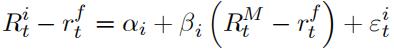
(b)From the previous steps, you must have 48 ![]() is and 48
is and 48 ![]() Plot the
Plot the ![]() with ±2SE?
with ±2SE?
Are the pricing errors (![]() ) big? What do you conclude?
) big? What do you conclude?
(c)Plotthe ![]() against E (
against E (![]() ) ; the latter computed as the unconditional mean of the excess return of industry i: The CAPM dictates that there must be a close relationship between the
) ; the latter computed as the unconditional mean of the excess return of industry i: The CAPM dictates that there must be a close relationship between the ![]() and the expected excess return. Do you observe such a relationship? What do you conclude?
and the expected excess return. Do you observe such a relationship? What do you conclude?
(d)Reconcilethe evidence in part b and c?

2.Let the returns on the SMB and HML portfolios be denoted by RSMBt andRHMLt,respectively. 金融计量经济学代写
Those factors have been proposed by Fama and French (1993) as additional risk factors. You will use the SMB and HML factors to see if they improve over the performance of the CAPM. Note that RSMBt and HMLt are already in excess of the risk free rate.
(a)For each asset, run the followingregression:

(b)From the previous steps, you must have ![]() . Plot the
. Plot the![]() with ±2SE? Are the pricing errors (
with ±2SE? Are the pricing errors (![]() ) big? How do the results compare to what you found in question 1.a.? What do you conclude?
) big? How do the results compare to what you found in question 1.a.? What do you conclude?
(c)Producethree graphs, plotting each of the ![]() against E (
against E (![]() ) ; the ticular, your first graph should plot the 48
) ; the ticular, your first graph should plot the 48 ![]() against E (
against E (![]() ) and should be directly comparable to what you obtained in question 1.b. Do you observe a relationship between excess returns and the various risk prices? Do you think that SMB and HML are priced factors? Why? Is a three-factor Fama-French model more suitable at capturing the fluctuation in equity returns? In answering the questions, refer to your empirical results. 金融计量经济学代写
) and should be directly comparable to what you obtained in question 1.b. Do you observe a relationship between excess returns and the various risk prices? Do you think that SMB and HML are priced factors? Why? Is a three-factor Fama-French model more suitable at capturing the fluctuation in equity returns? In answering the questions, refer to your empirical results. 金融计量经济学代写
(d)For an exact definition of the SMB and HML portfolios, go to the Fama and French (1993) article, or to http://mba.tuck.dartmouth.edu/pages/faculty/ken.french/Data_Library/f-html. Do you think that the SML and HMB returns are real risk factors? Why? Can you provide economic intuition to justify your answer? (HINT: Don’t spend too much time on this question.)
3.Pleaseread carefully through lecture notes 3 and 4.
更多代写:金融网课代修价格 代考英文 教育学网课代写 加拿大Essay怎么写 加拿大国际政治论文代写 英文代考
合作平台:essay代写 论文代写 写手招聘 英国留学生代写