Shooting method
计算机代考 Apply the Shooting Method to the nonlinear BVPs. Find a bracketing interval [s0,s1] and apply an equation solver to find and plot the ···
1.Carry out the steps of Computer Problem 1 for the BVPs 计算机代考
2.Apply the Shooting Method to the nonlinear BVPs. Find a bracketing interval [s0,s1] and apply an equation solver to find and plot the solution.
3.Carry out the steps of Computer Problem 3 for the nonlinear BVPs.
4.Apply the Shooting Method to the nonlinear systems of boundary value problems. Follow the method of Example 7.7.
Buckling of a Circular Ring 计算机代考
oundary value problems are natural models for structure calculations. A system of seven differential equations serves as a model for a circular ring with compressibility c, under hydrostatic pressure p coming from all directions. The model will be nondimensionalized for simplicity, and we will assume that the ring has radius 1 with horizontal and vertical symmetry in the absence of external pressure. Although simplified, the model is useful for the study of the phenomenon of buckling, or collapse of the circular ring shape. This example and many other structural boundary value problems can be found in Huddleston [2000].
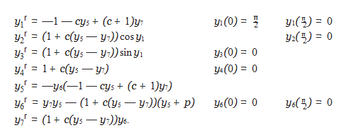
The model accounts for only the upper left quarter of the ring—the rest can be filled in by the symmetry assumption. The independent variable s represents arc length along the original centerline of the ring, which goes from s 0 to s π/2. The dependent variables at the point specified by arc length s are as follows:
y1(s) = angle of centerline with respect to horizontal
y2(s) = x-coordinate y3(s) = y-coordinate
y4(s) = arc length along deformed centerline
y5(s) = internal axial force y6(s) = internal normal force y7(s) = bending moment.
Figure 7.5(a) shows the ring and the first four variables. The boundary value problem (see, for example, Huddleston [2000]) is
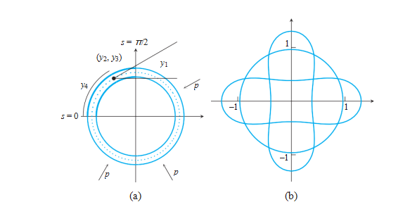
Figure 7.5 Schematics for Buckling Ring. 计算机代考
(a) The s variable represents arc length along the dotted centerline of the top left quarter of the ring. (b) Three different solutions for the BVP with parameters c =0.01, p =3.8. The two buckled solutions are stable.
Under no pressure (p 0), note that y1 π/2 s,(y2, y3) ( cos s, sin s), y4 s, y5
y6 y7 0 is a solution. This solution is a perfect quarter-circle, which corresponds to a perfectly circular ring with the symmetries.
In fact, the following circular solution to the boundary value problem exists for any choice of parameters c and p:
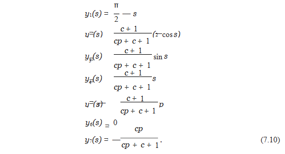
As pressure increases from zero, the radius of the circle decreases. As the pressure parameter p is increased further, there is a bifurcation, or change of possible states, of the ring. The circular shape of the ring remains mathematically possible, but unstable, meaning that small perturbations cause the ring to move to another possible configuration (solution of the BVP) that is stable.
计算机代考
For applied pressure p below the bifurcation point, or critical pressure pc, only solution (7.10) exists. For p > pc, three different solutions of the BVP exist, shown in Figure 7.5(b). Beyond critical pressure, the role of the circular ring as an unstable state is similar to that of the inverted pendulum (Computer Problem 6.3.6) or the bridge without torsion in Reality Check 6.
The critical pressure depends on the compressibility of the ring. The smaller the param- eter c, the less compressible the ring is, and the lower the critical pressure at which it changes shape instead of compressing in original shape. Your job is to use the Shooting Method paired with Broyden’s Method to find the critical pressure pc and the resulting buckled shapes obtained by the ring.
Suggested activities:
- Verifythat (7.10) is a solution of the BVP for each compressibility c and pressure p.
- Set compressibility to the moderate value c = 0. Solve the BVPby the Shooting Method for pressures p = 0 and 3. The function F in the Shooting Method should use the three missing initial values (y2(0), y5(0), y7(0)) as input and the three final values
(y1(π/2), y2(π/2), y6(π/2)) as output. The multivariate solver Broyden II from Chapter 2 can be used to solve for the roots of F . Compare with the correct solution (7.10). Note that, for both values of p, various initial conditions for Broyden’s Method all result in the same solution trajectory. How much does the radius decrease when p increases from 0 to 3?
- Plot the solutions in Step 2.The curve (y2(s), y3(s)) represents the upper left quarter of the ring. Use the horizontal and vertical symmetry to plot the entire ring.
- Change pressure to p = 3.5, and resolve the BVP. Note that the solution obtained depends on the initial condition used for Broyden’s Method. Plot each different solution found.
- Find the critical pressure pcfor the compressibility c = 0.01, accurate to two decimal places. For p > pc, there are three different solutions. For p < pc, there is only one solution (7.10).
- Carry out Step 5 for the reduced compressibility c = 0.The ring now is more brittle. Is the change in pc for the reduced compressibility case consistent with your intuition?
- Carryout Step 5 for increased compressibility c = 0.
FINITEDIFFERENCE METHODS 计算机代考
The fundamental idea behind finite difference methods is to replace derivatives in the differential equation by discrete approximations, and evaluate on a grid to develop a system of equations. The approach of discretizing the differential equation will also be used in Chapter 8 on PDEs.
Let y(t) be a function with at least four continuous derivatives. In Chapter 5, we developed discrete approximations for the first derivative

更多代写:C语言代写 北美考试代考 lab代写 本科essay代写 代包网课 数据建模代写