机器学习数据挖掘作业辅导-CS434代写-Machine Learning代写

CS434 Machine Learning and Data Mining – Homework 1

k-Nearest Neighbor Classifification and Statistical Estimation

机器学习数据挖掘作业辅导 Each question that you need to respond to is clearly marked in a blue “Task Box” with its corresponding point-value listed.

Overview and Objectives. In this homework, we are going to implement a kNN classififier and get some practice with the concepts in statistical estimation we went over in lecture. The assignment will help you understand how to apply the concepts from lecture to applications.

How to Do This Assignment. 机器学习数据挖掘作业辅导

Each question that you need to respond to is clearly marked in a blue “Task Box” with its corresponding point-value listed.

We prefer typeset solutions (LATEX / Word) but will accept scanned written work if it is legible. If a TA can’t read your work, they can’t give you credit. Submit your solutions to Canvas as a zip including your report and any code the assignment asks you to develop. You do not need to include the data fifiles.

Programming should be done in Python and numpy. If you don’t have Python installed in your machine, you can install it from https://www.python.org/downloads/. This is also the link showing how to install numpy:

https://numpy.org/install/. You can also search through the internet for numpy tutorials if you haven’t used it before. Google is your friend!

You are NOT allowed to…

Use machine learning package such as sklearn.
Use data analysis package such as panda or seaborn. 机器学习数据挖掘作业辅导
Discuss low-level details or share code / solutions with other students.

Advice. Start early. Start early. Start early. There are two sections to this assignment – one involving working with math (20% of grade) and another focused more on programming (80% of the grade). Read the whole document before deciding where to start.

How to submit. Submit a zip fifile to Canvas. Inside, you will need to have all your working code and hw1-report.pdf.You will also submit test set predictions to a class Kaggle competition. This is a required to receive credit for Q10.

Statistical Estimation [10pts] 机器学习数据挖掘作业辅导

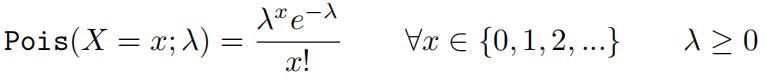
The Poisson distribution is a discrete probability distribution over the natural numbers starting from zero (i.e. 0,1,2,3,…).Specififically, it models how many occurrences of an event will happen within a fifixed interval. For example – how many people will call into a call center within a given hour. Importantly, it assumes that an individual event (a person calling the center) is independent and occurs with a fifixed probability. Say there is a 2% chance of someone calling every minute, then on average we would expect 1.2 people per hour – but sometimes there would be more and sometimes fewer. The Poisson distribution models that uncertainty over the total number of events in an interval.

The probability mass function for the Poisson with parameter λ is given as:

(1)

where the rate λ can be interpreted as the average number of occurrences in an interval. In this section, we’ll derive the maximum likelihood estimate for λ and show that the Gamma distribution is a conjugate prior to the Poisson.

Q1 Maximum Likelihood Estimation of λ [4pts]. Assume we observe a dataset of occurrence counts D = {x1, x2, …, x_N } coming from N i.i.d random variables distributed according to Pois(X = x; λ). Derive the maximum likelihood estimate of the rate parameter λ. To help guide you, consider the following steps:

Write out the log-likelihood function logP(D|λ).
Take the derivative of the log-likelihood with respect to the parameter λ.
Set the derivative equal to zero and solve for λ – call this maximizing valueˆλ MLE.

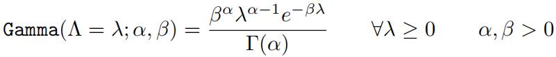
Your answer should make intuitive sense given our interpretation of λ as the average number of occurrences.In lecture, we discussed how to use priors to encode beliefs about parameters before any data is seen. We showed the Beta distribution was a conjugate prior to the Bernoulli – that is to say that the posterior of a Bernoulli likelihood and Beta prior is itself a Beta distribution (i.e. Beta ∝ Bernoulli * Beta) . The Poisson distribution also has a conjugate–the Gamma distribution. Gamma is a continuous distribution over the range [0, ∞) with probability density function:

(2)

Note that Γ(α) is referred to as the Gamma function whereas the overall expression represents the Gamma distribution.

Q2 Maximum A Posteriori Estimate of λ with a Gamma Prior [4pts].

As before, assume we observe a dataset of occurrence counts D = {x1, x2, …, xN } coming from N i.i.d random variables distributed ac-cording to Pois(X = x; λ). Further, assume that λ is distributed according to a Gamma(Λ = λ; α, β). Derive the MAP estimate of λ. To help guide you, consider the following steps:

Write out the log-posterior logP(λ|D) ∝ logP(D|λ) + logP(λ).
Take the derivative of logP(D|λ) + logP(λ) with respect to the parameter λ.
Set the derivative equal to zero and solve for λ – call this maximizing value ˆλMAP .

In the previous question we found the MAP estimate for λ under a Poisson-Gamma model; however, we didn’t demonstrate that Gamma was a conjugate prior to Poisson – i.e. we did not show that the product of a Poisson likelihood and Gamma prior results in another Gamma distribution (or at least is proportional to one).

Q3 Deriving the Posterior of A Poisson-Gamma Model [2pt]. Show that the Gamma distribution is a conjugate prior to the Poisson by deriving expressions for parameters αP , βP of a Gamma distribution such that P(λ|D) ∝ Gamma(λ; αP , βP ).

[Hint: Consider P(D|λ)P(λ) and group like-terms/exponents. Try to massage the equation to looking like the numerator of a Gamma distribution. The denominator can be mostly ignored if it is constant with re-spect to λ as we are only trying to show a proportionality (∝).]

2 k-Nearest Neighbor (kNN) [50pts]

In this section, we’ll implement our fifirst machine learning algorithm of the course – k Nearest Neighbors. We are considering a binary classifification problem where the goal is to classify whether a person has an annual income more or less than $50,000 given census information. Test results will be submitted to a class-wide Kaggle competition. As no validation split is provided, you’ll need to perform cross-validation to fifit good hyperparameters.

Data Analysis. We’ve done the data processing for you for this assignment; however, getting familiar with the data before applying any algorithm is a very important part of applying machine learning in practice. Quirks of the dataset could signifificantly impact your model’s performance or how you interpret the outcome of your experiments. For instance, if I have an algorithm that achieved 70% accuracy on this task – how good or bad is that? We’ll see! 机器学习数据挖掘作业辅导

We’ve split the data into two subsets – a training set with 8,000 labelled rows, and a test set with 2,000 unlabelled rows. These can be downloaded from the data tab of the HW1 Kaggle as “train.csv” and “test_pub.csv” respectively.Both fifiles will come with a header row, so you can see which column belongs to which feature.

Below you will fifind a table listing the attributes available in the dataset. We note that categorizing some of these attributes into two or a few categories is reductive (e.g. only 14 occupations) or might reinforce a particular set of social norms (e.g. categorizing sex or race in particular ways).

For this homework, we reproduced this dataset from its source without modifying these attributes; however, it is useful to consider these issues as machine learning practitioners.

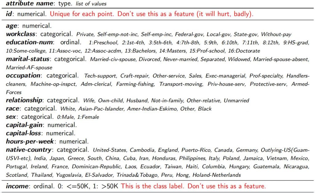
Our dataset has three types of attributes – numerical, ordinal, and nominal. Numerical attributes represent continuous numbers (e.g. hours-per-week worked). Ordinal attributes are a discrete set with a natural ordering, for instance difffferent levels of education. Nominal attributes are also discrete sets of possible values; however, there is no clear ordering between them (e.g. native-country). These difffferent attribute types require difffferent preprocessing. As discussed in class, numerical fifields have been normalized.

For nominal variables like workclass, marital-status, occupation, relationship, race, and native-country, we’ve trans-formed these into one column for each possible value with either a 0 or a 1. For example, the fifirst instance in the training set reads: [0, 0.136, 0.533, 0.0, 0.659, 0.397, 0, 0, 1, 0, 0, 0, 0, 0, 0, 0, 0, 1, 0, 0, 0, 0,0, 0, 0, 0, 0, 1, 0, 0, 0, 0, 0, 0, 0, 1, 0, 0, 0, 0, 0, 0, 0, 0, 1, 0, 0, 0, 0, 0, 0, 0, 0, 0, 0, 0, 0, 0, 0, 0, 0, 0, 0, 0, 0, 0, 0, 0, 0, 0, 0, 0, 0, 0, 0, 0, 0, 0, 0, 0, 0, 0, 1, 0, 0, 0,0] where all the zeros and ones correspond to these binarized variables. The following questions guide you through exploring the dataset and help you understand some of the steps we took when preprocessing the data. 机器学习数据挖掘作业辅导

Q4 Encodings and Distance [2pt] To represent nominal attributes, we apply a one-hot encoding tech-nique – transforming each possible value into its own binary attribute.

For example, if we have an attribute workclass with three possible values Private, State-gov, Never-worked – we would binarize the workclass at-tribute as shown below (each row is a single example data point):

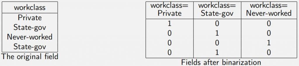
A common naive preprocessing is to treat all categoric variables as ordinal – assigning increasing integers to each possible value. For example, such an encoding would say 1=Private, 2=State-gov, and 3=Never-worked. Contrast these two encodings. Focus on how each choice affffects Euclidean distance in kNN.

Q5 Looking at Data [3pt] What percent of the training data has an income >50k? Explain how this might affffect your model and how you interpret the results. For instance, would you say a model that achieved 70% accuracy is a good or poor model? How many dimensions does each data point have (ignoring the id attribute and class label)? [Hint: check the data, one-hot encodings increased dimensionality]

2.1 k-Nearest Neighbors 机器学习数据挖掘作业辅导

In this part, you will need to implement the k-NN classififier algorithm with the Euclidean distance. The kNN algorithm is simple as you already have the preprocessed data. To make a prediction for a new data point, there are three main steps:

Calculate the distance of that data point to every training example.
Get the k nearest points (i.e. the k with the lowest distance).
Return the majority class of these neighbors as the prediction

Implementing this using native Python operations will be quite slow, but lucky for us there is the numpy package.numpy makes matrix operations quite effiffifficient and easy to code. How will matrix operations help us? The next question walk you through fifiguring out the answer. Some useful things to check out in numpy: broadcasting, np.linalg.norm np.argsort() or np.argpartition(), and array slicing.

Q6 Norms and Distances [2pt] Distances and vector norms are closely related concepts. For instance,an L2 norm of a vector x (defifined below) can be intepretted as the Euclidean distance between x and the zero vector:

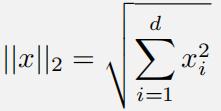(3)

Given a new vector z, show that the Euclidean distance between x and z can be written as an L2 norm.[kNN implementation note for later, you can compute norms effiffifficiently with numpy using np.linalg.norm] In kNN, we need to compute distance between every training example xi and a new point z in order to make a prediction. As you showed in the previous question, computing this for one xi can be done by applying an arithmetic operation between xi and z, then taking a norm.

In numpy, arithmetic operations between matrices and vectors are sometimes defifined by “broadcasting”, even if standard linear algebra doesn’t allow for them.For example, given amatrix X of size n × d and a vector z of size d, numpy will happily compute Y = X − z such that Y is the result of the vector z being subtracted from each row of X. Combining this with your answer from the previous question can make computing distances to every training point quite effiffifficient and easy to code.

Q7 Implement kNN Classifier [10pts] Okay, it is time to get our hands dirty. Let’s write some code! Implement k-Nearest Neighbors using Euclidean distance by completing the skeleton code provided in knn.py. Specififically, you’ll need to fifinish:

get_nearest_neighbors(example_set, query, k) 机器学习数据挖掘作业辅导

Given a n × d example_set matrix where each row represents one example point, return the indices of the k nearest examples to the query point. This is where the bulk of the computation will happen in your algorithm so you are strongly encouraged to review the paragraph above this task box to get hints for how to do it effiffifficiently in numpy.

knn_classify_point(examples_X, examples_y, query, k)

Given a n × d example_set matrix where each row represents one example point and a n × 1 column-vector with these points’ corresponding labels, return the prediction of a kNN classififier for the query point. Should use the previous function.

The code to load the data, predict for each point in a matrix of queries, and compute accuracy is already provided towards the end of the fifile. You’ll want to read over these carefully.

2.2 K-Fold Cross Validation 机器学习数据挖掘作业辅导

We do not provide class labels for the test set or a validation set, so you’ll need to implement K-fold Cross Validation¹to check if your implementation is correct and to select hyperpameters. As discussed in class, K-fold Cross Validation divides the training set into K segments and then trains K models – leaving out one of the segments each time and training on the others. Then each trained model is evaluated on the left-out fold to estimate performance. Overall performance is estimated as the mean and variance of these K fold performances.

Q8 Implement k-fold Cross Validation [8pts] Next we’ll be implementing k-fold cross validation by fifinishing the following function in knn.py:

cross_validation(train_X, train_y, num_folds, k)

Given a n × d matrix of training examples and a n × 1 column-vector of their corresponding labels,perform K-fold cross validation with num_folds folds for a k-NN classififier. To do so, split the data in num_folds equally sized chunks then evaluate performance for each chunk while considering the other chunks as the training set. Return the average and variance of the accuracies you observe.

For simplicity, you can assume num_folds evenly divides the number of training examples. You may fifind the numpy split and vstack functions useful.

Q9 Hyperparameter Search [15pt] To search for the best hyperpameters, run 4-fold cross-validation to estimate our accuracy. For each k in 1,3,5,7,9,99,999,and 8000, report:

accuracy on the training set when using the entire training set for kNN (call this training accuracy),
the mean and variance of the 4-fold cross validation accuracies (call this validation accuracy).

Skeleton code for this is present in main() and labeled as Q9 Hyperparmeter Search. Finish this code to generate these values – should likely make use of predict, accuracy, and cross_validation.

Questions: What is the best number of neighbors (k) you observe? When k = 1, is training error 0%? Why or why not? What trends (train and cross-valdiation accuracy rate) do you observe with increasing k? How do they relate to underfifitting and overfifitting? 机器学习数据挖掘作业辅导

2.3 Kaggle Submission

Great work getting here. In this section, you’ll submit the predictions of your best model to the class-wide Kaggle competition. You are free to make any modifification to your kNN algorithm to improve performance; however, it must remain a kNN algorithm! You can change distances, weightings, select subsets of features, etc.

1Note that K here has nothing to do with k in kNN – just overloaded notation.

Q10 Kaggle Submission [10pt]. Code at the end of main() outputs predictions for the test set to test_predicted.csv. Decide on hyperparameters and submit a set of predictions to Kaggle that outper-forms the baseline on the public leaderboard. Predictions are formatted as a two-column CSV as below:

id,income

0,0

1,0

2,0

3,0

4,0

5,1

6,0

You may submit up to 5 times a day. In your report, tell us what modififications you made to kNN for your fifinal submission. Note that the public leaderboard shows results on only half the test data, whereas a sepa-rate private leaderboard shows results for the whole set.

Extra Credit and Bragging Rights [2.5pt Extra Credit]. The TA has made a submission to the leader-board as well. Any submission outperforming the TA on the private leaderboard at the end of the homework period will receive 2.5 extra credit points on this assignment. Further, the top 5 ranked submissions will “win HW1” and receive bragging rights.

3 Debriefifing (required in your report) 机器学习数据挖掘作业辅导

Approximately how many hours did you spend on this assignment?
Would you rate it as easy, moderate, or diffiffifficult?
Did you work on it mostly alone or did you discuss the problems with others?
How deeply do you feel you understand the material it covers (0%–100%)?
Any other comments?

合作平台：essay代写论文代写写手招聘英国留学生代写