Mid-term test, November 5, 2020
Regression Analysis/MAT3375
Time: 2 hours (2:30 p.m.-4:30 p.m.)
回归分析考试代写 If a formula was proved in the lecture slides you do not need to prove it again. You can simply refer to page number in the lecture slides.
-
This exam is open book and should be completed at home indepen-dently. 回归分析考试代写
- Thesolution to this exam should be submitted on line in You can either print the exam and complete it or prepare your solutions on separate papers referring your solutions to each questions clearly. Please keep the order of questions as it is provided. Answer questions in separate pages. You can use your ipad or any other tablet co complete this test and submit in one single p.d.f. file. Make sure to use a thick pen so that the scan or photos of your solution is legible. You are not allowed to consult with any other individuals during the time you write this exam. The submitted mid-term should be in one single pdf file.
- Any conduct constitute cheating, misrepresenting, or unfairnessinclud-ing unauthorized aids and assistance, impersonating another person and committing plagiarism will be reported and will be dealt with based on regulations on code of conduct in academic matters. I will pick few students to interview about this exam.
- Write your detailed responses in the space provided. 回归分析考试代写
- At the end of exam you need to submit the test to brightspace.
- If you are registered with SASS, please email me your test. Add the additional time given to you based on the University of Ottawa’s rule and regulations.
- Where it is possible to check your work, do so.
- If you see any error in this exam, please report it on your paper.
- If a formula was proved in the lecture slides you do not need to prove it again. You can simply refer to page number in the lecture slides.
- Question 4 (3 points) is a bonus question.
- Youcan use any program you like in your computers for calculations.
[7]1.In a set of observations (x1, y1), . . . , (xn, yn) the regression model holds for(y |x ) i.∼i.d. N (g(x ), σ2).
In other words we can write
yi = g(xi) + si, i = 1, 2, . . . , n,
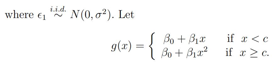
In here c is a known constant. Derive M.L.E. for β0, β1 and σ2. Calculate the distribution for βˆ0 and βˆ1, the M.L.E. estimators for β0 and β1.
[8]2.We believe the dataset
(1, 2), (0, 0), (−1, 0), (1, 3), (2, 5), (−2, 2), (−1, −1).
The model
yi = βxi + x2 + si
is suggested. How do you estimate β using the least square estimator? As- suming s i.∼i.d. N (0, σ2), derive the distribution for βˆ, the L.S.E. for β, and construct a 95% confidence interval for β.

3.The following R output considers 4 models with two predictors x1and x2.
Model 1, is the following full model
yi = β0 + β1xi1 + β2xi2 + si, i = 1, 2, . . . , 13.
> X
x1 x2
[1,] 1 -1.80010433 -0.5405582
[2,] 1 -0.04229331 -1.3709413
[3,] 1 -0.08678218 0.2957614
[4,] 1 0.06111548 0.9415597
[5,] 1 1.14330745 2.5285609
[6,] 1 1.92056231 1.6081196 回归分析考试代写
[7,] 1 1.82138798 0.5624988
[8,] 1 2.75304245 1.6156332
[9,] 1 3.44569675 1.8407098
[10,] 1 3.65246789 3.9496973
[11,] 1 4.85153144 3.8753938
[12,] 1 3.71436981 5.3106420
[13,] 1 5.12777189 3.9816031
> y
[1] -1.2891234 0.7065793 7.6110556 3.5745170 3.5235997 3.9997938
[7] 8.5709438 1.2894697 13.7879403 13.0325041 13.1410099 13.9692036
[13] 15.6586959
%%%%%%%%%%%%%%%%%%%%%%%%%%%%%%%%%%%%%%%%%%%%%%%%%%%%%%%%%%%%%%%%%%%%%%%%%%%%
> solve(t(X)%*%X)
x1 x2
0.16099642 -0.02126662 -0.02146733
x1 -0.02126662 0.06290956 -0.05669175
x2 -0.02146733 -0.05669175 0.07256185
%%%%%%%%%%%%%%%%%%%%%%%%%%%%%%%%%%%%%%%%%%%%%%%%%%%
> cor(x1,y)
[1] 0.8311754
> cor(x2,y)
[1] 0.7697804
%%%%%%%%%%%%%%%%%%%%%%%%%%%%%%%%%%%%%%%%%%%%%%%%%%%%%
> model1=lm(y~x1+x2)
> anova(model1)
Analysis of Variance Table
Response: y
Df Sum Sq Mean Sq F value Pr(>F) 回归分析考试代写
x1 1 288.075 288.075 23.7033 0.000653 ***
x2 1 7.376 7.376 0.6069 0.453994
Residuals 10 121.534 12.153
—
Signif. codes: 0 *** 0.001 ** 0.01 * 0.05 . 0.1 1
%%%%%%%%%%%%%%%%%%%%%%%%%%%%%%%%%%%%%%%%%%%%%%%%%%%%%%%%%%%%%%%%%%%%%%%%%%%
> model2=lm(y~x1)
> anova(model2)
Analysis of Variance Table
Response: y
Df Sum Sq Mean Sq F value Pr(>F)
x1 1 288.07 288.075 24.582 0.0004301 ***
Residuals 11 128.91 11.719
—
Signif. codes: 0 *** 0.001 ** 0.01 * 0.05 . 0.1 1
> model3=lm(y~x2)
> anova(model3)
Analysis of Variance Table
Response: y
Df Sum Sq Mean Sq F value Pr(>F) 回归分析考试代写
x2 1 247.09 247.089 15.998 0.002087 **
Residuals 11 169.90 15.445
%%%%%%%%%%%%%%%%%%%%%%%%%%%%%%%%%%%%%%%%%%%%%%%%%%%%%%%%%%%%%%%%%%%
> model4=lm(y~x1-1)
> anova(model4)
Analysis of Variance Table
Response: y
Df Sum Sq Mean Sq F value Pr(>F)
x1 1 970.71 970.71 65.195 3.42e-06 ***
Residuals 12 178.67 14.89
—
Signif. codes: 0 *** 0.001 ** 0.01 * 0.05 . 0.1 1
%%%%%%%%%%%%%%%%%%%%%%%%%%%%%%%%%%%%%%%%%%%%%%%%%%%%%%%%%%%%%%%%%%
> model1$coef
(Intercept) x1 x2
2.5576359 1.7442504 0.7315846
> model2$coef
(Intercept) x1 回归分析考试代写
2.774074 2.315829
> model3$coef
(Intercept) x2
3.147281 2.303438
1
2.99818
%%%%%%%%%%%%%%%%%%%%%%%%%%%%%%%%%%%%%%%%%%%%%%%%%%%%%%%%5
[5] (i) Use the R out put to construct a 95% confidence interval for β0 in model 1. Use this confidence interval to test 回归分析考试代写
H0 : β0 = 0 against H1 : β0 ƒ= 0
at α = 5% level.
[5] (ii) Which model do you suggest to use based on the R output? Justify your answer statistically in few statements. Write your final suggested model in a Mathematical form. Write the M.L.E. for parameters of your final model and explain why your suggested model is preferred.
[3 points (bonus)] 4. Label each statement as True or False. Justify your answers very briefly. 回归分析考试代写
(i)If E(y|x) = a + bx, then (x, y) follow a bivariate normal distribution.
(ii)If (x, y) follows a bivariate normal distribution, then both
V ar(y|x) and V ar(x|y)
are free from x and y.
(iii)If x‘ = [x1 x2 · · xn] ∼ Nn(0, Σ) then both xj Σx and xj Σ−1x have χ2(n) distributions.
更多代写:美国EconFinal exam代考 雅思代考 网课代修靠谱推荐 留学生英文essay论文写作 留学生作业essay代写 essay写手费用
合作平台:essay代写 论文代写 写手招聘 英国留学生代写