Walmart Sales Forecasting Final Report
商业分析报告代写 The aim of this project is to predict the weekly department-wise sales of 45 Walmart stores in the US using historical data
Problem
The aim of this project is to predict the weekly department-wise sales of 45 Walmart stores in the US using historical data
The ability to forecast sales for any business is of crucial importance. With an insight on what the expected sales would be in the near future the businesses can plan accordingly. The managers are able to schedule shifts, allocate resources, stock inventory etc based on the forecast.
The dataset is taken from Kaggle from a competition hosted by Walmart.
Client 商业分析报告代写
A lot of businesses have a somewhat homogenous sales trend over time except for in the Holiday seasons. Being able to accurately predict the sales in the Holiday seasons is even more important. The challenge in predicting Holiday sales is that there isn’t much data available. This problem can be applied to any industry/business whose sales are affected by the holiday seasons. They can use this information to manage resources, complete inventory, launch applicable promotions etc.
Dataset
The data that I will be using is of 45 Walmart stores. The dataset can be easily downloaded from Kaggle. It contains department wise weekly sales for each store for over 2 years, along with 12 features.
The data in available as 4 tables:
- Train Sales – Store wise department wise weekly sales for 2 years
- Test Sales – Store, department and dates
- Features – This contains the stores region characteristics like fuel price, temperature,
Consumer affluence, unemployment percentage and active promotions over time
- Store – This defines the type and size of each store. 商业分析报告代写
The columns descriptions are:
- Store – the store number
- Dept – the department number
- Date – the week
- Weekly_Sales – sales for the given department in the given store (Only present in train data)
- IsHoliday – whether the week is a special holiday week
- Type – Description not given
- Size – Description not given but is self explanatory
- Temperature – average temperature in the region
- Fuel_Price – cost of fuel in the region
- MarkDown1-5 – anonymized data related to promotional markdowns that Walmart is running.
MarkDown data is only available after Nov 2011, and is not available for all stores all the time.
- CPI – the consumer price index
- Unemployment – the unemployment rate
Data Wrangling
First, we input data & perform data wrangling. We conduct the following steps to clean up the data
- Joining the tables:
○ We join the tables together to get all the features in one table. The final table
resulted in a total of 15 Features for 415,000 observations in the training data.
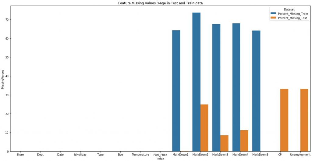
- Missing values.
○ There were some features which had upto 70% of the value’s missing. Such features were made redundant.
○ Other features with fewer missing values were zero-imputed.
○ Some features were missing only in the test data.
3. Negative Sales
○ It was observed that 0.305 percent of the target feature(Weekly_sales) were negative.
○ The competition posters(Walmart) have not given any reason as to why that would be.A logical reasoning would be that these would be weeks where the returns were
more that the sales for these weeks in these departments.
Other than the issues highlighted the data is mostly clean. 商业分析报告代写
Exploratory Data Analysis
Note: The problem that we are trying to solve is fundamentally a time-series problem. To convert this into a conventional time series problem we need to find/develop/extract features that depict the Weekly_Sales trend over time.
During exploratory data analysis, we ask the following conclusions were observed:
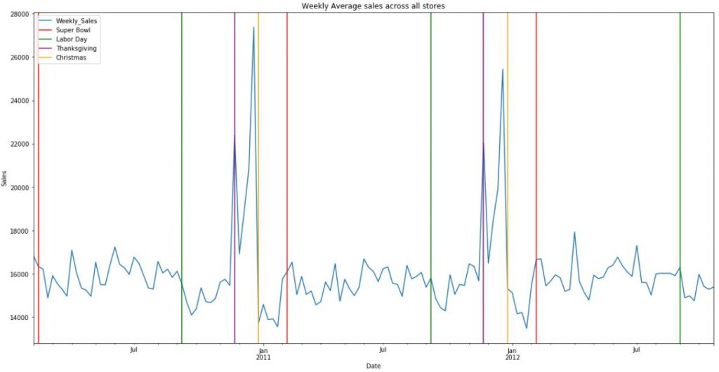
- Weekly_Sales trend is affected by some holidays but not all.
a.Thanksgiving and Christmas holidays affect Weekly Sales more than Superbowl and Labor Day.
b.The sales sharply drop after all holidays except SuperBowl.
c.There is an offset in the weekly_sales for christmas.
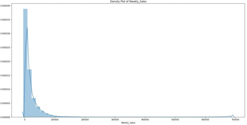
2. The target variable (Weekly_Sales) is NOT normally distributed.
a.The distribution of weekly_Sales is very skewed. This limits the effectiveness of most of the parametric machine learning models which rely on the assumption that the
distribution is normal.
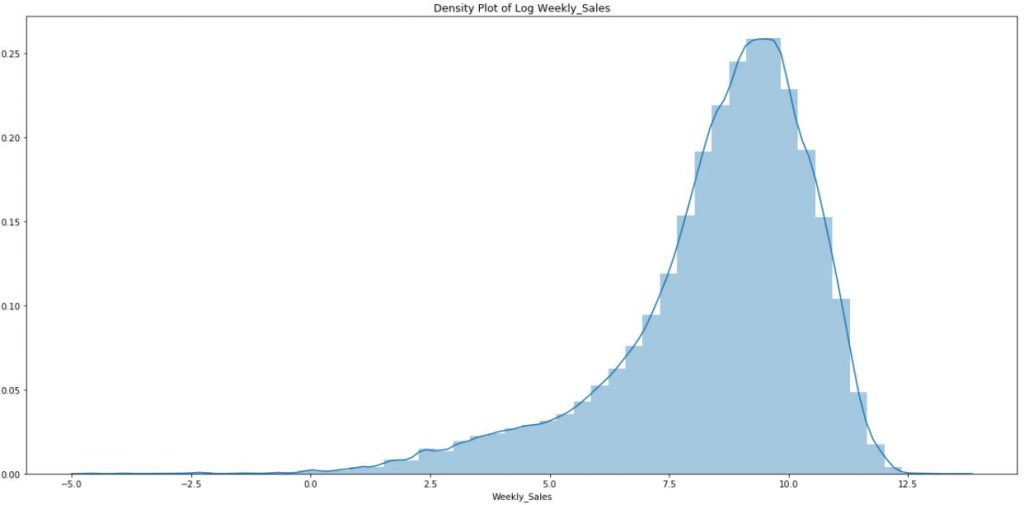
b.Log transformed Weekly_Sales is a lot less skewed and seemed close to normal.However, this assumption was negated after performed a statistical test to prove normality.
3. Most important features in predicting Weekly_Sales 商业分析报告代写
a.Upon performing some analysis on the data set the following features emerged as being the most reasonably correlated with Weekly_Sales.
Most of these features were either extracted or engineered.
i.CPI_Cat and Size_Cat: CPI (Customer Propensity Index) and Size (of Store) were available in the training data as continuous values. These were discretized following along the rational that came from the Exploratory Data analysis.
ii.Which_holiday: The training data had a column for ‘IsHoliday’. It was realized during EDA that each holiday had a different trend on the weekly sales. Some holidays had virtually no effect on the sales trends e.g. Labor Day as shown below. As a result feature was created for each holiday
iii. TillNext{Holiday}, SinceNext{Holiday}: These features were created to depict the number of weeks since a particular holiday has passed and the number of weeks until the next holiday comes. These were created for 4 holidays thus a total of 8 features
iv.DateLagFeatures: This feature depicts the Weekly Sales for each Store-Dept pair ‘x’ weeks from the current week. 商业分析报告代写
v.DateFeatures: This features were derived from the date of the observation. These include,Quarter,Month,Year,WeekOfMonth,WeekOfYear. viDepartment_Contribution: This feature is the ratio of each Department’s average monthly sales with the Store’s average monthly sales. The rational here is that the ratio would be a measure of how much the department’s sales contribute to the sales of the store for each month.
vii. Store_dept_month_avg: This is the average sale for that store,dept pair for that month
4.Consistency of each department’s sales trends
a.Upon visual inspection of the sales trend of a department across different Stores it was observed that most departments show similar trends if normalized against the stores total sales volume.
5.Redundant features
It was observed that all the features other than the ones mentioned above showed very weak correlation with the Weekly_Sales and thus were discarded.
Takeaways
From the analysis we can conclude the following:
i.Weekly Sales should be transformed to the logarithmic scale so that the distribution isn’t as skewed
ii.Weekly sales outliers problem is somewhat sorted by transforming to the logarithmic scale, however, there might still be need to look into outliers that appear after the scale change. This can be done in the modeling process
iii. Its best to use non parametric algorithms to solve the problem since they are less affected by the features or the target variable being not normal

Statistical Analysis 商业分析报告代写
Statistical tests were performed to assess the following:
- Series Stationarity
○ The test concluded that the series is NOT stationary
- AutoCorrelation
○ The weekly_sales are highly correlated with the previous 4 week’s sales. The
highest correlation is with last years week.
- Relationships of some features with Weekly_Sales
○ Features with weak relationships were discarded as a result.
Takeaways
- Additional transformations will need to be made if using Time-Series based techniques
- The previous weeks sales can be used as a feature
Modeling strategy:
I tried to solve the problem using an ensemble of 3 models. The final results were the average of the prediction from each model.
Model 1: XGBoost Model trained all of the training data.
Model 2: XGBoost Models trained on each Store-Dept pair
Model 3: RandomForest Models trained on each Store-Dept pair.
Model 1 – Single XGB Model:
This model is an Xtreme Gradient Boosting regressor trained on all of the training data.
Following is a list and description of the features that were engineered to generate optimal results. 商业分析报告代写
Features Engineered:
- CPI_Cat and Size_Cat: CPI (Customer Propensity Index) and Size (of Store) were available in the training data as continuous values. These were discretized following along the rational that came from the Exploratory Data analysis.
- Which_holiday:The training data had a column for ‘IsHoliday’. It was realized during EDA that each holiday had a different trend on the weekly sales. Some holidays had virtually no effect on the sales trends e.g. Labor Day as shown below. As a result feature was created for each holiday
- TillNext{Holiday}, SinceNext{Holiday}: These features were create to depict the number of weeks since a particular holiday has passed and the number of weeks until the next holiday comes. These were created for 4 holidays thus a total of 8 features
- DateLagFeatures: This feature depicts the Weekly Sales for each Store-Dept pair ‘x’weeks from the current week. 商业分析报告代写
- DateFeatures:This features were derived from the date of the observation. These include, Quarter,Month,Year,WeekOfMonth,WeekOfYear
- Department_Contribution: This feature is the ratio of each Department’s average monthly sales with the Store’s average monthly sales. The rational here is that the ratio would be a measure of how much the department’s sales contribute to the sales of the store for each month.
- Store_dept_month_avg: This is the average sale for that store,dept pair for that month
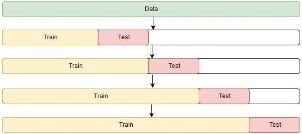
The model was trained the XGBRegressor API. Sample weights were included in the training according to where the observation fell in a Holiday or not. The model for tuned using GridSearchCV using a 4-fold Time series train,test scheme as shown below:
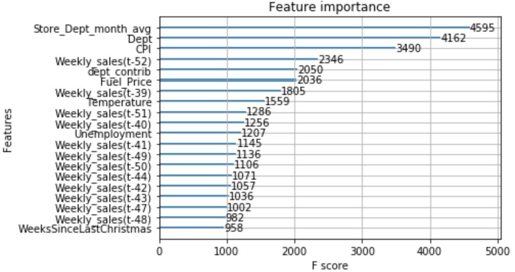
The following is a plot of the top 20 most important features from the final model.
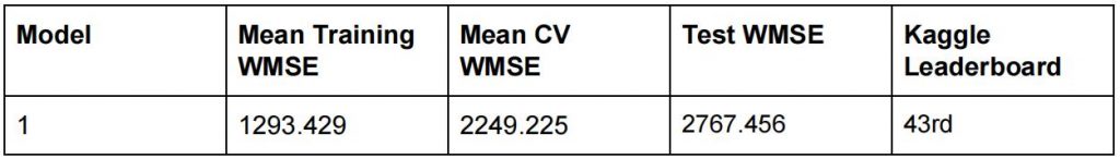
Results:
The models were evaluated using the Weighted Mean Absolute Error where the weight is 5 for Holiday dates
Model 2 – Granular XGB Models:
This approach is more granular that Model 1. A different model was trained for each Store-Dept pair. If less than 10 observations were available in the data for any pair than all the data for that Department was used. The rationale for this approach is that according to EDA the sale trends for all Departments were similar across all Stores. This observation implies that every department sells the same things, irrespective of the Store. Thus, it would make sense to train a model for each Store-Dept pair.
The target for transformed to log(Weekly_Sales) so that a near normal distribution could be simulated. It proved faster to train with better results. 商业分析报告代写
Lesser amount of features were engineered for this approach since now each model will have considerably less samples to train so adding more features would have caused problems in the line of curse of dimensionality.
- CPI_cat and Size_cat: Similar to the ones in Model 1
- Date_features
- LagSales for 5 weeks
3 Fold – TImeSeries cross validation was used to tune the models.
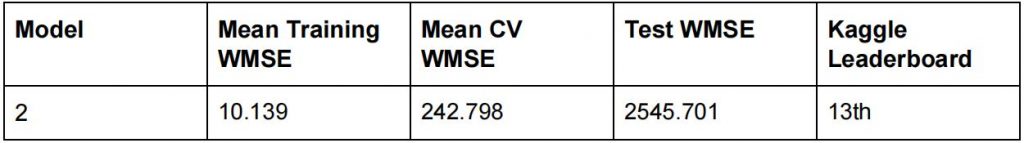
Results:
Model 3: Granular RF Models:
Same as Model 2 but used RandomForest instead of XGB model.
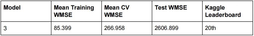
Results:
Post Adjustment:
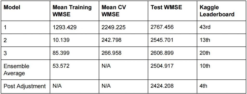
I averaged the results of these models to make the final prediction.
One observation that was noted in data; In the first year of the training data, Christmas occurs on a Saturday (with weeks ending on Friday). That causes all of its sales bulge to fall into the week before. In the second year of the training data, it occurs on a Sunday, so there is one pre-Christmas shopping day in week 52. The test set has Christmas for 2012 which puts it on a Tuesday, with 3 pre-Christmas shopping days in its week.
I implemented a post-forecast adjustment that said that if, in a given department, the average sales for weeks 49, 50 and 51 were at least 10% higher than for weeks 48 and 52, than I would circularly shift a particular fraction of the sales from weeks 48 through 52 into the next week (and from 52 back to 48).Since the underlying model is based on 2 years of data, I shifted 2.5/7. This is because the test year shifts 2 days with respect to the second year of the training data, and 3 days with respect to the first year.
Final Results:Model
Error Analysis
The following is a heatmap of the errors department-Store errors
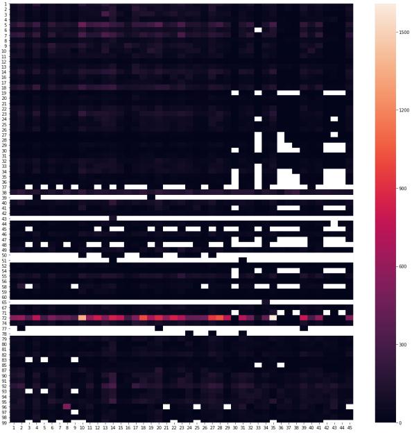
We can see that the models are not performing well for department 72. The maximum error is on store 10, department 72.
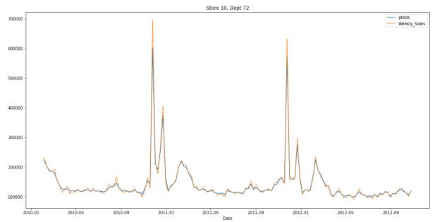
On first sight it seems that the predictions are really good. The problem here is that it is a very high Sales pair. The average sales for this store is more than 10 times the average of all the stores. Thus,even a slight deviation from the actual values results in a high error. One remedy could be to train separate models for such stores.
Conclusion: 商业分析报告代写
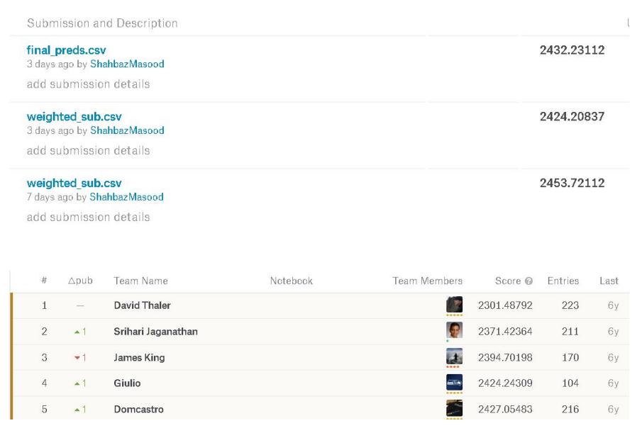
The above approach to forecast sales of store is successful. The results have put me on the 4th position on Kaggle. This approach can be used to forecast the sales of any company for which salesforcasting is crucial for their operations, especially during the Holiday season.
Further Improvements:
- Models for the poor performing departments can be analysed individually to be tuned further
- The RF models have room for further tuning but it takes a lot of time to train.
- The threshold for the post adjust can also be tuned. As of now 10% was chosen arbitrarily.
- The granular models approach, though effective, is not very efficient. In production environments it would be a difficult task to manage them.
更多代写:代上统计学网课 代考托福 网课代托 代写Essay结构 代写写作技巧 代写履历
合作平台:essay代写 论文代写 写手招聘 英国留学生代写