博客

Physics 281: Computational Physics

Homework Set 5

Computational Physics作业代写 When everything is working, you will have three curves lying almost exactly on top of each other, and therefore impossible to see.

Reading

• Newman Ch. 5: Integrals and Derivatives. You should carefully read Sec. 5.1: Fundamental methods for evaluating integrals. Then, read Secs. 5.2 through 5.9 for an understanding of how the scipy.integrate functions we will be using work.
• Handout Summary of numerical methods, through the section “Numer- ical Integration”.
• You will find these homework problems much easier if you complete the activities for 3/14-15/19 first.

Homework problems  Computational Physics作业代写

Each problem counts for 10 points. Full credit for this set = 30 points (do at least all the un-starred problems). Hints and tricks are in a separate section Coding Hints after the homework problems.

1.Computing Bessel functions. If you are not familiar with Bessel functions,take a quick look at the Wikipedia article on  For this problem, plot J₁(x) computed three different ways on the same plot, over the range 0 ≤ x ≤ 20:

(a)Use the special function forJ₁(x).

(b)Compute J₁(x) from its integralrepresentation

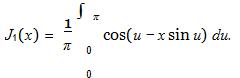
Use your own code to evauate this integral using the trapezoid rule or Simpson’s rule (your choice) (not using the trapezoid or Simpson’s integrators in scipy.integrate).

12019-03-22 P281 HW5.tex §c 2019 Donald Candela

(c)Again compute J₁(x) from the integral representation, but now useintegrate.quad() to evaluate the the integral.  Computational Physics作业代写

When everything is working, you will have three curves lying almost exactly on top of each other, and therefore impossible to see. To fix this,add small offsets (whatever is enough to see all three curves clearly) to the second and third curves. Your plot should have a legend explaining what is what including what offsets are used.

2. Newman 5.4(b): The diffraction limit of a telescope. Make a density plot showing the diffraction pattern, as Newman requests. For this plot, compute J₁(x) from its integral representation, with the integral evaluated using scipy.integrate.quad().  Computational Physics作业代写
3. Newman 5.9: Heat capacity of a solid. Look at the Wikipedia article Debye model to see what your graph should look like. Again use scipy.integrate.quad() to evaluate the integral, rather than using Gaussian quadrature. The point is that scipy.integrate.quad() is a good general-purpose integrator that will automatically pick a numer- ical method suitable for many types of problem. Programming notes:

• Put everything in SI units: V in m³, k_Bin J/K, etc. For example, rho   =   022e28 #  number   density   of   aluminum   (m^-3) Then C_V will come out in J/K. Be sure to label the axes of your plot including units.

4. *Newman 5.14: Gravitational pull of a uniform sheet (double integral example) Rather than using double Gaussian quadra- ture as Newman requests, use scipy.integrate.dblquad which is a general-purpose double integrator.

Coding Hints  Computational Physics作业代写

Hints and tricks that you might find helpful:

• Computing Bessel functions.

-For parts 1b and 1c, the function that defines the integrand for thenumerical integral depends both on the integration variable u and also the parameter x (the point at which J₁(x) is being evaluated), for example:

def fj1(u,x):

“””Integrand for computing J1(x).”””

return cos(u – x*sin(u))

For part 1b you can handle this by writing a Simpson’s-rule inte- gration function that takes the extra argument x:  Computational Physics作业代写

def simps(f,a,b,nn,x):

“””Simpson’s-rule integration of  f(u,x)du  from  a  to  b  using  nn  points # now the value of x is available to use when this

# function calls fj1(u,x)

…

return …

For part 1c there is an optional argument to scipy.integrate.quad() for this very purpose, passing additional arguments to the inte- grand function. The option is args=(..) as shown here:

def j1quad(x):

“””J1(x) computed using scipy.integrate.quad.””” return (1/pi)*quad(fj1,0,pi,args=(x))[0]

We need [0] on the end because scipy.integrate.quad() re- turns a pair of numbers, the result and the accuracy, and we only want the first of these. This code will call fj1(..) with two ar- guments, the integration variable and the additional argument x.

– For parts 1b and 1c, you will get an error if you try to vectorize the caculation of J₁(x). This won’t work:

xpts = 100    Computational Physics作业代写

x = np.linspace(0,20,xpts)

yquad = j1quad(x) # vectorized like this doesn’t work

Instead you will need to compute J₁(x) point by point:

xpts = 100

x = np.linspace(0,20,xpts)

yquad = np.zeros(xpts) # so do point-by-point for j in range(xpts):

yquad[j] = j1quad(x[j])

• The diffraction limit of a telescope.

• You should be able to re-use your code for computing J₁(x) us- ing integrate.quad() from the previous problem. Once again, you will need to compute the image array point by point rather thanvectorizing.
• Recallyou cannot use lambda as a variable name; it means some- thing else in Python.
• You can ignore Hint 1 in Newman if you want, but you will get a divide-by-zerowarning if one of your image points is right at the origin.

• Gravitational pull of a uniform sheet.  Computational Physics作业代写

To evaluate the double integral

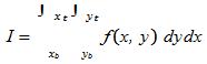
the code is

I =

x_b y_b

f (x, y) dydx

from scipy.integrate import dblquad

def  f(y,x): # note y comes first here! “””Integrand.”””

return …

def ybot(x):

return yb def ytop(x):

return yt

ii = dblquad(f,xb,xt,ybot,ytop) # do the double integral

This form with functions ybot(x) and ytop(x) is used to allow you to make the y-limits depend upon x, which is needed for more complicated problems (but not this one).

更多代写：代修网课多少钱  雅思枪手  代做java  电影专业report代写  法律毕业论文代写  Appeal Letter怎么写

合作平台：essay代写 论文代写 写手招聘 英国留学生代写