Intro to AI. Assignment 1
Summer 2022
1.1 Probabilistic reasoning
Suppose that each day when driving to campus, there is a 1% chance that my children have a meltdown, and that when my children have a meltdown, there is a 98% chance that I will be late. On the other hand, even when my children do not have a meltdown, there remains a 3% chance that I will be late for other reasons (e.g., traffic).
Suppose that one day I am late to campus. What is the probability that my children had a meltdown? Use Bayes rule to compute your answer, and show your work.

1.2 Conditioning on background evidence AI作业代写
It is often useful to consider the impact of specific events in the context of general background evidence, rather than in the absence of information. Denoting such evidence by E, prove the following variants of Bayes rule and marginalization:
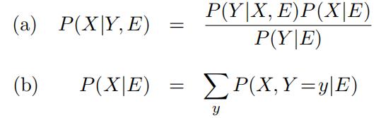
1.3 Conditional independence
Show that the following three statements about random variables X, Y , and E are equivalent:
(i)P (X, Y |E) =P (X|E)P (Y |E)
(ii)P (X|Y, E) = P(X|E)
(iii)P (Y |X, E) =P (Y |E)
In other words, show that each one of these statements implies the other two. You should become fluent with all these ways of expressing that X is conditionally independent of Y given E.
1.4 Creative writing AI作业代写
Attach events to the binary random variables X, Y , and Z that are consistent with the following patterns of commonsense reasoning. You may use different events for the different parts of the problem.
(a)Explainingaway:
P (X = 1|Z = 1) > P (X = 1),
P (X = 1|Y = 1, Z = 1) < P (X = 1|Z = 1)
(b)Accumulatingevidence:
P (X = 1) < P (X = 1|Y = 1) < P (X = 1|Z = 1, Y = 1) AI作业代写
(c)Conditionalindependence:
P (X, Y |Z) = P (X|Z)P (Y |Z),
P (X = 1, Y = 1) < P (X = 1)P (Y = 1).
1.5 Probabilistic inference
Recall the probabilistic model that we described in class for the binary random variables E = Earthquake, B = Burglary, A = Alarm, J = JamalCalls, M = MayaCalls . We also expressed this model as a belief network, with the directed acyclic graph (DAG) and conditional probability tables (CPTs) shown below:
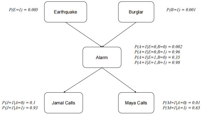
Compute numeric values for the following probabilities, exploiting relations of marginal and conditional independence as much as possible to simplify your calculations. You may re-use numerical results from lecture (for example, parts (a) and (c) will be discussed in lecture), but otherwise show your work. Be careful not to drop significant digits in your answer.
(a) P (B = 1|A = 1) (c) P (A = 1|J = 1) (e) P (A = 1|M = 0)
(b) P (B = 1|A = 1, E = 0) (d) P (A = 1|J = 1, M = 1) (f) P (A = 1|M = 0, E = 1)
Consider your results in (b) versus (a), (d) versus (c), and (f) versus (e). Do they seem consistent with commonsense patterns of reasoning?
1.6 Kullback-Leibler distance AI作业代写
Often it is useful to measure the difference between two probability distributions over the same random variable. For example, as shorthand let
pi = P (X = xi|E),
qi = P (X = xi|Ej)
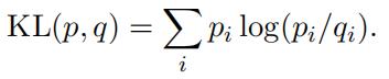
denote the conditional distributions over the random variable X for different pieces of evidence E ≠ E‘. Note that both distributions satisfy ![]() The Kullback-Leibler (KL) distance between these distributions is defined as:
The Kullback-Leibler (KL) distance between these distributions is defined as:
(a)Bysketching graphs of log z and z − 1, verify the inequality
log z ≤ z − 1,
with equality if and only if z = 1. Confirm this result by differentiation of log z (z 1). (Note: all logarithms in this problem are natural logarithms.)
(b)Use the previous result to prove thatKL(p, q) 0, with equality if and only if the two distributions pi and qi are equal. Hint: substitute z = qi/pi into the previous inequality. AI作业代写
(x)Providea simple numerical counterexample to show that the KL distance is not a symmetric function of its arguments:
KL(p, q) ĭ KL(q, p).
Despite this asymmetry, it is still common to refer to KL(p, q) as a measure of distance between prob- ability distributions.
更多代写:Computer Architecture代写 悉尼pte代考 包网课机构 Persuasive Speech代写 Reflection paper 代写 essay的introduction怎么写
合作平台:essay代写 论文代写 写手招聘 英国留学生代写