Time series forecasting for Brooklyn, NY rental prices using SARIMA and Holt-Winters methods
环境艺术类代写 Rents in some Brooklyn neighborhoods are nearing or exceeding those in Manhattan [1]. Rising rents impact families and low-income New Yorkers.
1. Introduction 时间序列作业代写
Brooklyn, NY has become an increasingly popular rental area over the past decade. Rents in some Brooklyn neighborhoods are nearing or exceeding those in Manhattan [1]. Rising rents impact families and low-income New Yorkers. StreetEasy, a New York City real estate site, has produced a number of studies on affordability of housing in New York. Rents for NYC listed on StreetEasy have increased by 31% overall between January 2010 and January 2018
[2] with some Brooklyn neighborhoods growing over 40% [3]. Without considering the implications of COVID-19, I’ve generated two models, seasonal ARIMA and seasonal Holt-Winters, to forecast the median rental prices in Brooklyn, NY into the first half of 2021.

2. Data set
StreetEasy captured the median rental prices in NYC from January 2010 to March 2020 [4]. Initially, I included all rental types and boroughs in the data set. After taking steps to clean the data (see Appendix.1), I narrowed the analysis to two bedrooms in Brooklyn. Fig.1 gives a sense for the raw and cleaned data.
Fig.1 (a) raw data all rental types and boroughs from StreetEasy
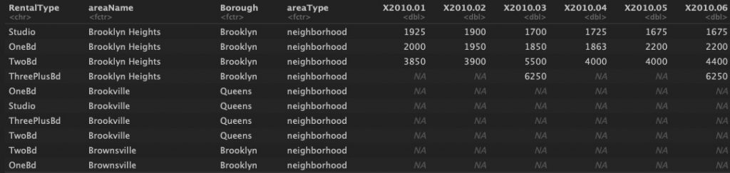
Fig.1 (b) cleaned data 2bd Brooklyn data
3. Results 时间序列作业代写
3.1Visualize, evaluate pattern of thedata
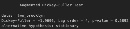
From the plot of the time series data (see Fig. 2), the data does not appear stationary. There is a logarithmic trend with an upward swing around 2018 and potential seasonality. To confirm trend and seasonality, I plotted a classical decomposition chart (see Fig. 3) and performed a Dickey-Fuller test (see Appendix.2) to check for a drift in the mean of the data (unit root). From the classical decomposition, there is a clear trend and seasonal pattern to the data and because the data is monthly the seasonal period is 12. The Dickey-Fuller test produced a p-value of 0.5892, so I did not reject the null hypothesis that the time series is non-stationary.
Fig. 2
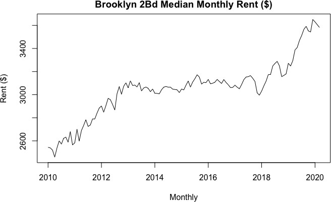
Fig. 3
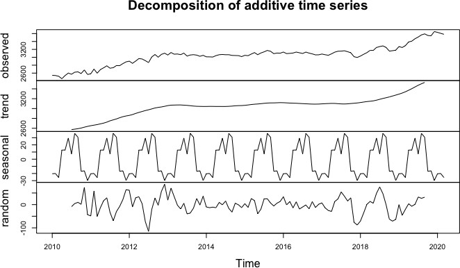
Fig. 3
3.2Transformations
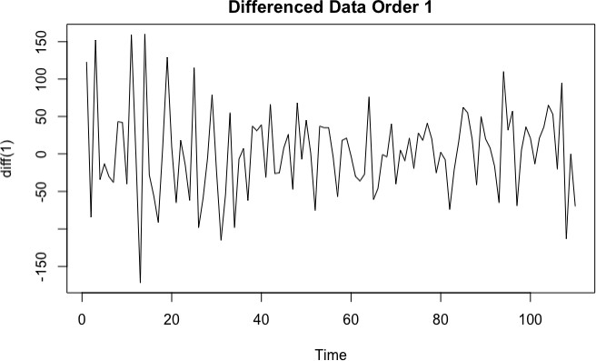
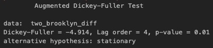
To correct for seasonality (deterministic part) and unit root, I applied a difference of order 1 and order 12 (see Fig. 4).
A variance stabilizing transformation was not needed. The p-value after rerunning the Dickey-Fuller test was 0.01 indicating stationarity (see Appendix.3).
Fig. 4
3.3Model-based Forecast: ARIMA
To forecast future values of the time series, I used a seasonal ARIMA model. The model-based approach fits an ARIMA model to data to then forecast. From the ACF and PACF plots (see Fig. 5), it seems reasonable to consider a low order ARMA model. The PACF cuts off near lag 2 decaying to 0 and the ACF cuts off after lag 2 decaying to 0. However, although there is an early cutoff, the lag significance returns around month 12 and this periodic pattern is a characteristic of seasonality with period 12 (stochastic part). This confirms what was observed in the seasonal component from Fig.3. 时间序列作业代写
Fig. 5
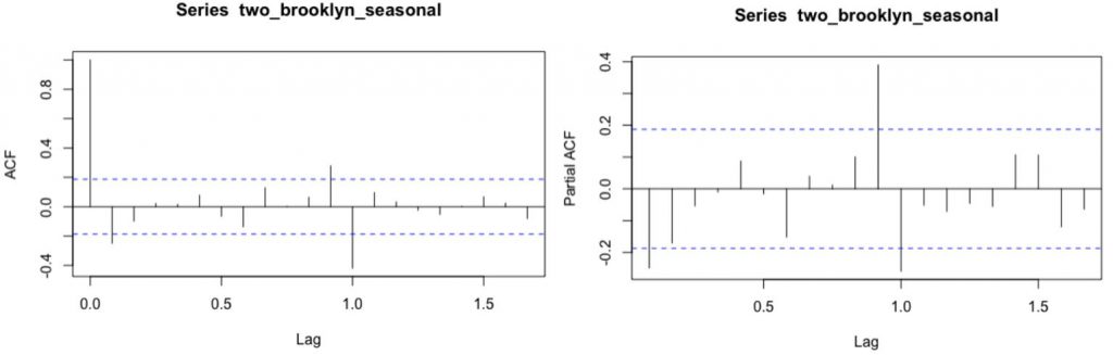
For the initial model, I chose an ARMA (2,1,2) x SARMA (1,1,1)12 model. First, for the non-seasonal ARMA(p,d,q) model, there is a decaying pattern in the ACF and PACF. Second, for the seasonal ARMA(P,D,Q) model, there is strong autocorrelation and strong partial autocorrelation around lag 12 and both cutoff decaying to 0. Because there are multiple interpretations to take, I generated six additional variations and compared performance. Although the different models had roughly comparable AICc values (see Table.1), the initial model had the smallest and that was the model that was used for forecasting the time series (see Fig. 6).Fig. 5
Table.1 AICc values per ARIMA model
| Model | AICc |
| (2,1,2) x (1,1,1)[12] | 1170.18 ** |
| (2,1,2) x (0,1,1)[12] | 1173.43 |
| (2,1,1) x (0,1,1)[12] | 1171.84 |
| (2,1,0) x (0,1,1)[12] | 1170.62 |
| (1,1,0) x (1,1,1)[12] | 1172.49 |
| (2,1,1) x (1,1,1)[12] | 1174.23 |
| (1,1,1) x (0,1,1)[12] | 1171.8 |
Fig.6

3.4ModelDiagnostics 时间序列作业代写
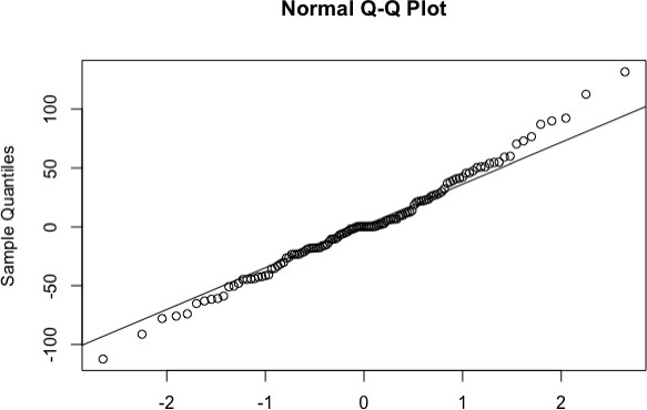
The ARMA (2,1,2) x SARMA (1,1,1)12 model had the lowest AICc value, the Q-Q plot shows that the data is coming from a normal population (see Appendix.4), and diagnostic plots indicate that the ACF of the residuals and p-values are not significant, so the model is adequate (see Fig. 7).
Fig. 7 model diagnostics
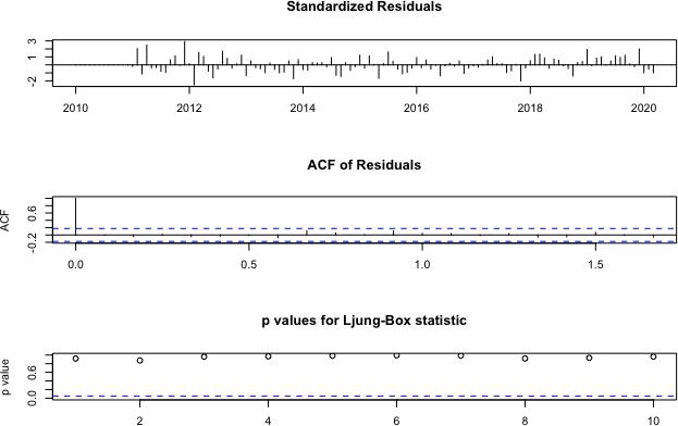
The majority of the model parameters were also significant. Of the 6 parameters in the model, 4 non-seasonal AR(2) MA(2) and 2 seasonal SAR (1) SMA(1), 4 seasonal parameters were significant while only the seasonal SMA(1) was significant (see Appendix.5). Taking out the non-significant SAR(1) parameter in the ARMA (2,2) x SARMA (0,1)12 model did not improve the AICc value (see Table.1).
3.5 Smoothing-based Forecast:Holt-Winters
Another widely used and successful forecasting method is the seasonal Holt-Winters method. The smoothing-based method uses the pattern of the data to extrapolate the forecast using double exponential smoothing. I performed the additive version as the seasonal pattern remained roughly the same for the range of the data. The forecast looks reasonable (see Fig. 8).
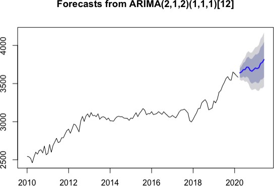
Fig. 8 Holt-Winters forecast of 2bd Brooklyn
3.6 Evaluation of ForecastAccuracy 时间序列作业代写
Both the seasonal ARIMA and seasonal Holt-Winters models look reasonable, but forecast accuracy is an important aspect in determining an appropriate model. To judge forecast accuracy, I used an out-of-sample forecast validation to compare the two methods. My validation sample size was about 11% of the total sample size or the 14 most recent observations. With seasonal data, it is important to hold back enough of the seasonality in the test sample.
I used the root mean square error (RMSE), Mean Absolute Error (MAE), and Mean absolute Percentage Error (MAPE) measures to evaluate the forecast. After running the metrics, the seasonal ARIMA model performed better than the seasonal Holt-Winters (see Table.2).
Table.2
| Holt-Winters | SARIMA (2,1,2) x (1,1,1)[12] | |
| MAE | 209.729741 | 192.759418 |
| RMSE | 232.326900 | 218.947107 |
| MAPE | 5.895694 | 5.609597 |
4. Conclusions
The purpose of this time series analysis was to forecast the rental prices of Brooklyn NY into the first half of 2021. I used the seasonal ARIMA and seasonal Holt-Winters models for forecasting rent from April 2020 to June 2021 (see Appendix.6). Then, I chose the suitable forecasting method by considering the AICc values among the ARIMA models and RMSE, MAE, and MAPE when comparing against the Holt-Winters method. The results showed that the seasonal ARIMA model can represent a suitable forecasting method for rental prices. This model can be extended to the other boroughs of New York City. For future analysis, it would also be interesting to include an intervention methodology anticipating some threshold of COVID-19 impact on NY rents as new rental listings fell 52% in the second half of March [5].
REFERENCES: 时间序列作业代写
- https://streeteasy.com/blog/february-2020-market-reports/
- https://furmancenter.org/research/sonychan
- https://streeteasy.com/blog/nyc-rent-affordability-2018/#_ftn1
- https://streeteasy.com/blog/data-dashboard/
- https://streeteasy.com/blog/q1-2020-market-reports/
APPENDIX
[1]
A few steps were taken to clean the raw data in Fig.1 for analysis.
a.Rows were removed where there were more than 3 consecutive NA values and remaining NAs replaced with last-observation-carried-forward method. This is a common approach when accounting for NAs.
b.In order to structure the data to perform time series analysis, I converted the column headers (example X2010.01) into date values. I then transformed the data into a single record per year per month by rental type and borough.
[2]
[3]
[4]
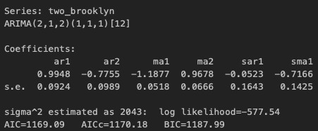
[5]ARMA (2,1,2) x SARMA (1,1,1)12 estimated parametervalues
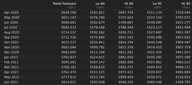
[6]ARMA (2,1,2) x SARMA (1,1,1)12 forecastedvalues
更多代写:环境艺术类代写 线上考试作弊 北美PHIL哲学代写 实验报告怎么写 论文标题格式 response怎么写
合作平台:essay代写 论文代写 写手招聘 英国留学生代写