
CSCI E-106:Assignment 2
数据建模作业代写 Students should submit their reports on Canvas. The report needs to clearly state what question is being solved, step-by-step walk-through
Due Date: September 21, 2020 at 7:20 pm EST
Instructions
Students should submit their reports on Canvas. The report needs to clearly state what question is being solved, step-by-step walk-through solutions, and final answers clearly indicated. Please solve by hand where appropriate.
Please submit two files: (1) a R Markdown file (.Rmd extension) and (2) a PDF document, word, or html generated using knitr for the .Rmd file submitted in (1) where appropriate. Please, use RStudio Cloud for your solutions.
Problem 1 数据建模作业代写
Refer to the regression model Yi = β0 + si. (25pts)
a-) Derive the least squares estimator of β0 for this model.(10pts)
Q = (Yi − b0)2 dQ = −2 ∗ (Yi − b0) = (Yi) − nb0 = 0 b0 = Y
b-) Prove that the least squares estimator of β0 is unbiased.(5pts)
Y N (β0, σ2 ) E(b0) = E(Y ) = β0
c-) Prove that the sum of the Y observations is the same as the sum of the fitted values.(5pts)
Σ Yˆ = Σ Y = nY = n Σ Yi = Σ Y
d-) Prove that the sum of the residuals weighted by the fitted values is zero.(5pts)
Σ Yˆiei = Σ Y (Yi − Yˆi) = Y Σ(Yi − Y ) = 0
Problem 2
Refer to the Grade point average Data. The director of admissions of a small college selected 120 students at random from the new freshman class in a study to determine whether a student’s grade point average (GPA) at the end of the freshman year (Y) can be predicted from the ACT test score (X). (30 points, each part is 5 points)
a-) Obtain a 99 percent confidence interval for β1. Interpret your confidence interval. Does it include zero? Why might the director of admissions be interested in whether the confidence interval includes zero?
99% confidence interval is 0.0054 ≤ β1 ≤ 0.072. It did not include zero, indicating that β1 is significant.

## 0.5% 99.5%
## (Intercept) 1.273902675 2.95419590 数据建模作业代写
## X 0.005385614 0.07226864
b-) Test, using the test statistic t∗, whether or not a linear association exists between student’s ACT score (X) and GPA at the end of the freshman year (Y). Use a level of significance of α = 0.01. State the alternatives,decision rule, and conclusion.
H0 : β1 = 0 Ha : β1 = 0 From the summary table below, t∗=3.04 and p value is 0.00292 < α = 0.01. Reject,
H0. You can alternatively, calculate the critical value of the test, the p value of the test directly, please see below.
summary (f.gpa)
##
## Call:
## lm(formula = Y ~ X, data = GPA) ##
## Residuals:
## Min 1Q Median 3Q Max ## -2.74004 -0.33827 0.04062 0.44064 1.22737 ##
## Coefficients:
## Estimate Std. Error t value Pr(>|t|)
## (Intercept) 2.11405 0.32089 6.588 1.3e-09 ***
## X 0.03883 0.01277 3.040 0.00292 ** ## —
## Signif. codes: 0 ‘***’ 0.001 ‘**’ 0.01 ‘*’ 0.05 ‘.’ 0.1 ‘ ‘ 1 ##
## Residual standard error: 0.6231 on 118 degrees of freedom
## Multiple R-squared: 0.07262, Adjusted R-squared: 0.06476 ## F-statistic: 9.24 on 1 and 118 DF, p-value: 0.002917
qt(1-0.01/2,118)
## [1] 2.618137
2*(1–pt(3.04,118))
## [1] 0.002914602
c-) What is the P-value of your test in part (b)? How does it support the conclusion reached in part (b)? see above, part b.
d-)Obtain a 95 percent interval estimate of the mean freshman GPA for students whose ACT test score is 28. Interpret your confidence interval.
Estimated GPA for ACT score of 28 is 3.2. 95% confidence interval for ACT=28 is 3.06 ≤ ttP A ≤ 3.34.
predict(f.gpa,data.frame(X=28),interval=“confidence”,level=0.95)
## fit lwr upr ## 1 3.201209 3.061384 3.341033
e-) Mary Jones obtained a score of 28 on the entrance test. Predict her freshman GPA-using a 95 percent prediction interval. Interpret your prediction interval. Estimated GPA for ACT score of 28 is 3.2. 95% confidence interval for ACT=28 is 1.96 ≤ ttP A ≤ 4.44.
predict(f.gpa,data.frame(X=28),interval=“prediction”,level=0.95, se.fit = FALSE)
## fit lwr upr ## 1 3.201209 1.959355 4.443063
f-) Is the prediction interval in part (e) wider than the confidence interval in part (d)? Should it be? 数据建模作业代写
Yes, it is wider. The prediction interval will be always wider than confidence interval as the variance is larger for the prediction interval.
g-) Determine the boundary values of the 95 percent confidence band for the regression line when Xh =28.Isyour-confidence band wider at this point than the confidence interval in part (d)? Should it be?W 2 = 2F (1 = α; 2, n − 2) = 2F (0.95; 2, 118) = 2(3.07) = 6.1462 W = 2.4792; 3.2012 − 2.4792 ∗ 0.0706 ≤β0 + β1Xh ≤ 3.2012 − 2.4792 ∗ 0.0706 3.0262 ≤ β0 + β1Xh ≤ 3.3762
predict(f.gpa,data.frame(X=28),interval=“confidence”,level=0.95,se.fit=TRUE)
## $fit
## fit lwr upr ## 1 3.201209 3.061384 3.341033 ##
## $se.fit
## [1] 0.07060873 ##
## $df
## [1] 118 ##
$residual.scale
## [1] 0.623125
W2= 2*qf(1-0.05,2,118)
W=sqrt(W2)
W
## [1] 2.479149
cbind(3.2012–2.4792*0.0706,3.2012+2.4792*0.0706)
## [,1] [,2]
[1,] 3.026168 3.376232

Problem 3 数据建模作业代写
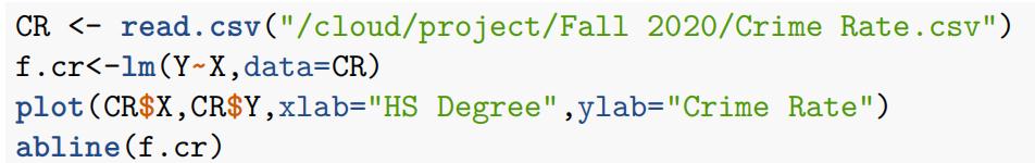
Refer to the Crime rate data. A criminologist studying the relationship between level of education-and crime rate in medium-sized U.S. counties collected the following data for a random sample of 84 counties; X is the percentage of individuals in the county having at least a high-school diploma, and Y is the crime rate (crimes reported per 100,000 residents) last year. (45 points, each part is 5 points)
a-)Obtain the estimated regression function. Plot the estimated regression function and the data. Does the linear regression function appear to give a good fit here? Discuss.
No it does not look like a good fit. High School gradation rate is not a strong variable. The other variables are missing such as unemployment rate, income and etc.
b-) Test whether or not there is a linear association between crime rate and percentage of high school graduates, using a t test with α = 0.01. State the alternatives, decision rule, and conclusion. What is the P-value of the test?
H0 : β1 = 0 Ha : β1 = 0 From the summary table below, t∗=-4.103 and p value is 0.00009 < α = 0.01. Reject,
H0. You can alternatively, calculate the critical value of the test, the p value of the test directly, please see below.
summary(f.cr)
##
## Call:
## lm(formula = Y ~ X, data = CR) ##
## Residuals:
## Min 1Q Median 3Q Max ## -5278.3 -1757.5 -210.5 1575.3 6803.3 ##
## Coefficients:
## Estimate Std. Error t value Pr(>|t|)
## (Intercept) 20517.60 3277.64 6.260 1.67e-08 ***
## X -170.58 41.57 -4.103 9.57e-05 *** ## —
## Signif. codes: 0 ‘***’ 0.001 ‘**’ 0.01 ‘*’ 0.05 ‘.’ 0.1 ‘ ‘ 1 ##
## Residual standard error: 2356 on 82 degrees of freedom ## Multiple R-squared: 0.1703, Adjusted R-squared: 0.1602 ## F-statistic: 16.83 on 1 and 82 DF, p-value: 9.571e-05 数据建模作业代写
qt(0.01/2,82)
## [1] -2.637123
2*pt(–4.103,82)
## [1] 9.567866e-05
c-) Estimate β1, with a 99 percent confidence interval. Interpret your interval estimate.
99% confidence interval is −280.22 ≤ β1 ≤ −60.94. It did not include zero, indicating that β1 is significant.
confint(f.cr,level=0.99)
## 0.5 99.5
## (Intercept) 11874.0517 29161.14822
## X -280.2118 -60.93856
d-) Set up the ANOVA table. see below
anova(f.cr)
## Analysis of Variance Table ##
## Response: Y
## Df Sum Sq Mean Sq F value Pr(>F)
## X 1 93462942 93462942 16.834 9.571e-05 ***
## Residuals 82 455273165 5552112 ## —
## Signif. codes: 0 ‘***’ 0.001 ‘**’ 0.01 ‘*’ 0.05 ‘.’ 0.1 ‘ ‘ 1
e-) Carry out the test in part a by means of the F test. Show the numerical equivalence of the two test statistics and decision rules. Is the P-value for the F test the same as that for the t test? 数据建模作业代写
H0 : β1 = 0 Ha : β1 ƒ= 0
From the ANOVA table above, F ∗ = 16.834 and p value is 0.000001 alpha=0.01. Reject H0, β1 is significant. Yes the p values are the same.
f-) By how much is the total variation in crime rate reduced when percentage of high school graduates is introduced into the analysis? Is this a relatively large or small reduction?
Total Variation is variation of Y is 548,736,107. It was reduced by SSR, the part that explained by the X, 93,462,942 or 93462942/548736107 or 17%.
(length(CR$Y)–1)*var(CR$Y)
## [1] 548736108
g-) State the full and reduced models.
Full model is Yi = β0 + β1Xi Reduced model is Yi = β0
h-) Obtain (1) SSE(F), (2) SSE(R), (3) dfF. (4) dfR, (5) test statistic F* for the general linear test, (6) decision rule.
From the ANOVA Table above
(1) SSE(F)=455273165
(2) SSE(R)=548736107 数据建模作业代写
(3)dfF=82
(4)dfR=83
H0 : β1 = 0 Ha : β1 ƒ= 0
![]()
The test is rejected as the pvalue is less than 0.01 or 16.834 ≥ 6.95
{(548736107-455273165)/(83-82)}/(455273165/82)
## [1] 16.83376
1–pf(16.834,1,82)
## [1] 9.570412e-05
qf(0.99,1,82)
## [1] 6.95442
i-)Are the test statistic F* and the decision rule for the general linear test numerically equivalent to those in part a?
Yes, they are equivalent.
更多代写:Matlab代写多少钱 Gre代考 英国网课代上代修 Definition Essay代写 毕业论文代做 网课代修机构