Physics 281: Computational Physics, Spring 2019 Activities for Meetings 14-15, Tues-Thurs 3/19-21/191
代写留学生物理 print out the integral computed three ways so they can be com- pared– the exact result, using quad, and using your trapezoid-rule integration.
Reading
Newman Ch. 5: Integrals and Derivatives. You should carefully read Sec. 5.1: Fundamental methods for evaluating integrals. Then, read Secs. 5.2 through 5.9 for an understanding of how the scipy.integrate functions we will be using work.
Handout Summary of numerical methods, through the section “Numer- ical Integration”.
In-Class Activities
Completing all of the non-starred activities will count as A-level work. To receive credit, these activities must be checked off in class or office hours within three weeks (by Fri 4/12).
1. Practice using complex numbers in Python.
(a)Please recall how you divide complexnumbers: 代写留学生物理

On a piece of scratch paper work out the real and imaginary parts of z = (3 + 4i)/(5 + 6i) using the formula above, then show that (3+4j)/(5+6j) in Python gives the same thing.2
(b)Inphysics you will make a lot of use of Euler’s formula:

These formulas work fine for both real and complex z (and please remember that 1/i = i). On a piece of scratch paper use the formulas above to compute the following quantities: e2i, cos(3i). Then show that exp(2j), cos(3j) computed by Python agree with your results.
12019-03-17 P281 W8ab.tex c 2019 Donald Candela
2The parentheses are necessary here because Python recognizes 4j and 6j on their own as complex numbers – try it without them to see what happens. 代写留学生物理
(c)Assumez = x + iy where x and y are real, and time t is Use Euler’s formula to compute the real and imaginary parts of eizt. Then, define a python function that computes f (t) = eizt where
z = ..+..j is set in your program outside of the function f (t). Your function should simply use exp (not Euler’s formula) and it will return a complex value.
Finally, set z = 5.0+0.2i and use your function to make two plots: First, plot Re[f (t)] and Im[f (t)] vs t as two curves on the same plot, for 0 < t < 10. Then, on a separate figure plot Im[f (t)] on the y-axis vs Re[f (t)] on the x-axis over the same range of t. This second plot will look better if you make the figure square.
Explain why these two plots look the way they do.
Coding hint: If t is your array of real t values and ft is your array of complex f (t) values, then you do the first plot with plt.plot(t,ft.real,…)
plt.plot(t,ft.imag,…)
and the second plot with
plt.figure(…) # start new plot, set figure size/shape plt.plot(ft.real,ft.imag,…)
2.Numerical integration using integrate.quad. You can eas- ily showthat 代写留学生物理
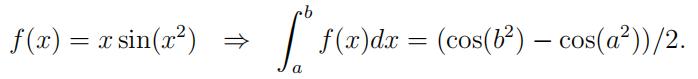
Write a program that computes and prints out ∫ 5 f (x)dx two different ways:
(a)theexact result using the worked-out integral on the right above, and
(b)using integrate.quad to evaluate the integral numeri- cally.

3.Numerical integration: Trapedzoid rule. This continuesactiv- ity Add to your program, so that it will repeatedly 代写留学生物理
(a)askthe user for the number of slices N to use for numerical com- putation (you could make your program quit if N < 1 is entered),
(b)usethe trapezoid rule with N slices to evaluate the integral, and
(c)print out the integral computed three ways so they can be com- pared– the exact result, using quad, and using your trapezoid-rule integration.
By running your program, find out how large N must be for the trapezoid-rule integration (a) to compute the integral to six-digit ac- curacy, and if possible (b) to compute the integral to the full number of digits in the “exact” calculation. 代写留学生物理
Coding suggestion: I suggest you write a function trap(f,a,b,nn) to do a trapezoid-rule integration of the function f from a to b with nn slices. This function will come in handy for this activity, as well as future activities and homework problems. You can either use the code in Newman, or (better) use the vectorized code discussed in class.
4.Numerical integration: Simpson’s rule.
Continuing the previous activity,write a function simps(f,a,b,nn) to do a Simpson’s-rule in- tegration of the function f from a to b with nn This function willl not be much different than your trapezoid-rule function, but it should not allow the number of slices to be odd – if given an odd N it should either print an error message, or do something to make N even (or both).
Have your program print out the result from your Simpson’s-rule inte- gration along with the earlier results, and answer the same questions about the value of N needed as for the previous activity.
5.Computing and plotting a function defined by an integral. 代写留学生物理
Considerthe following function (you can prove this using integration by parts):
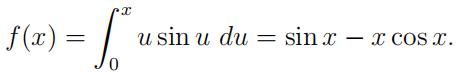
Plot f (x) over the range 0 < x < 20 three different ways, as three curves on the same plot (with a legend):
(a)Plotthe RHS of the equation above.
(b)Compute the integral above using scipy.integrate.quad.
(c)Computethe integral above using Simpson’s rule.
You should end up with three curves right on top of each other. To see the curves more clearly, add small constants to two of the curves to separate the curves slightly and modify your plot legend accordingly,
e.g. plt.plot(…,label=’integral using quad + 5’). 代写留学生物理
Check how small you can make the number of slices N before the Simpson’s-rule curve to looks noticeably wrong – the answer is surpris- ingly small, I think.
Coding hints:
- To do the Simpson’s-rule integration you can use the function simps discussed above for Activity 4.
- You cannot vectorize the calculation of the curves for quad and for Simpson’s rule, in other words this will not work :
x = np.linspace(0,20,pts)
ysimp = simps(f,0,x,nn)
Instead, you must compute the plotting array point by point:
x = np.linspace(0,20,pts)
ysimp = np.zeros(pts) # make array to hold Simpsons results for j in range(pts): # for each x point,
ysimp[j] = simps(f,0,x[j],nn) # compute integral for that x
The reason is that both quad and your simps function have things inside them like if statements that do not vectorize. 代写留学生物理
Remember that quad does not return a number – it returns a tuple of two numbers, the integral and the error estimate. You just want the first of these. You can pick out the first element using indexing, by putting [0] on the end:
yquad[j] = quad(f,0,x[j])[0]
or you can do this with a comma and and an underscore:
yquad[j],_ = quad(f,0,x[j])
The underscore _ by itself is a valid variable name. Customarily it is only assigned to values that will not be used later, like the error estimate in this case.
6.*Double integrals. 代写留学生物理
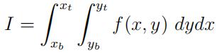
Double and triple integrals come up fairly of- ten in physics. The Python functions integrate.dblquad and scipy.integrate.tplquad are available to evaluate them numerically. Hereyou should try out dblquad on a double integral you can do ana- lytically, for example
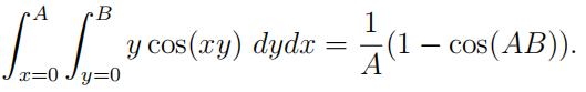
To evaluate the double integral
the code is
from scipy.integrate import dblquad
def f(y,x): # note y comes first here! “””Integrand.”””
return …
def ybot(x):
return yb def ytop(x): 代写留学生物理
return yt
ii = dblquad(f,xb,xt,ybot,ytop) # do the double integral
This form with functions ybot(x) and ytop(x) is used to allow you to make the y-limits depend upon x, which is needed for more complicated problems (but not this one).
For this activity, use dblquad to evaluate I(A, B) for a few sets of A, B values and compare with the analytical result above (feel free to substitute some other double integral you know how to do). I found that dblquad worked well for A, B ≤ 25, but not for bigger values– probably because the factor cos(xy) in the integrand has too many oscillations.
更多代写:美国统计网课代上 加拿大雅思代考 纽约大学网课代修 留学生英语essay写作 论文写作润色 sas作业代做价格
合作平台:essay代写 论文代写 写手招聘 英国留学生代写