代做应用统计-Applied Statistics代写-ECS764P代写

Applied Statistics (ECS764P) – Lab 4

代做应用统计 The following code will download and plot the entire world GDP time series. Do NOT make any local copies of your data!

1 Theory 代做应用统计

1.Consider the measure d on {1, 2, 3} × {1, 2, 3} defifined by

d(1, 1) = 1/10

d(1, 2) = 2/10

d(1, 3) = 1/10

d(2, 1) = 1/10

d(2, 2) = 1/10

d(2, 3) = 2/10

d(3, 1) = 1/10

d(3, 2) = 0

d(3, 3) = 1/10

(where I’ve written d(x, y) for d ({(x, y)}) in order to keep things readable.)

(a) Is d a probability measure?

(b) Prove that d cannot be written as a product measure. Hint: prove it by contradiction.

(d) Compute the covariance and correlation of d.

You can assume that numpy, matplotlib, scipy and pandas-datareader are installed on the machine of the person who will run and mark your notebook. There is no need to force an install with the ! command. For textual answers please use a markdown cell.

1.You will fifirst download the world GDP data from the World Bank using (which we used in lab 2). The following code will download and plot the entire world GDP time series. Do NOT make any local copies of your data!

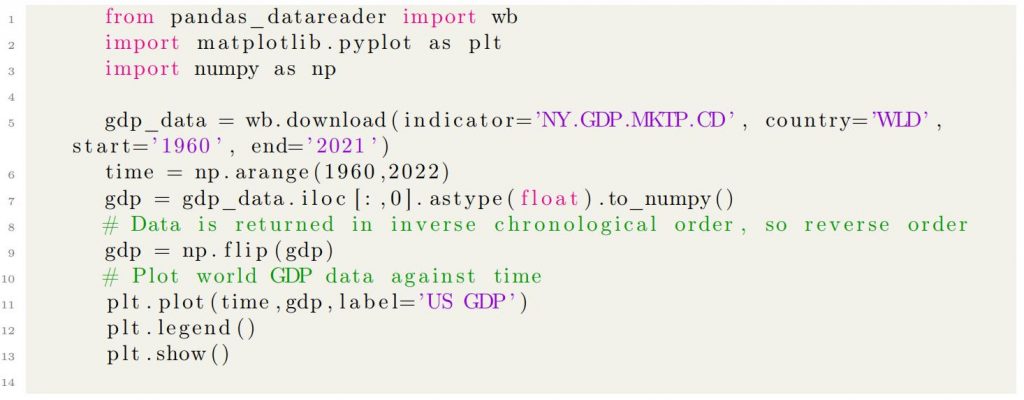
(you can ignore the warning about the code ‘WLD’). You will try to estimate the long-term annual growth rate of the world using a regression.

If the growth rate was a constant r, then the world’s GDP would grow as GDPk = GDP0(1 + r) k

where k is the number of years since 1960 and GDP0 is the world’s GDP in 1960. This is clearly not a linear relationship between time (k, in years) and GDP. However, we can get a linear relationship by applying a simple transformation f(−) on both side of the equation. What is this transformation?

(Hint: we used this transformation in the context of MLE, it turns products into sums.)

Apply this transformation f(−) to the GDP data, and perform a regression against the time variable. On the same plot, display your regression line, a scatter-plot of the (transformed) data points, and your R2 value.

You will now apply the inverse of the transformation f(−) to your linear model in order to get a non-linear model for the GDP. On the same plot, display your (non-linear) model and a scatter-plot of the (original) data points. 代做应用统计

What is the relationship between the slope of the regression and the long-term growth rate of the world GDP? Compute the long-term growth rate of the world GDP.

What do you observe since approximately 2015?

2. Download the Dow Jones Industrial Average from Yahoo fifinance using the following code. Do NOT make any local copies of your data!

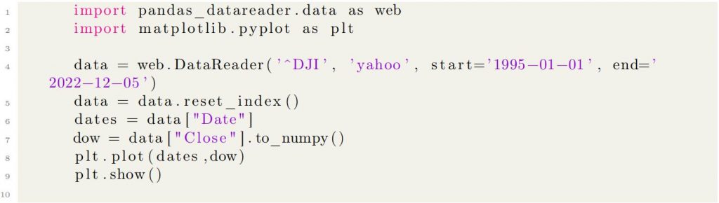
You will study the autocorrelation of this time series.

Instantiate an array lags=[1,2,3,5,10,15,20,30]. For each lag in lags compute and plot the history of the 60-day rolling autocorrelation of dow. Make your plot(s) legible.

For each lag in lags, compute the average of the autocorrelation times series computed in the previous step and use these 8 values to plot the autocorrelation function (autocorrelation against lag). What do you observe? Does this plot suggest that the Dow Jones is a white noise process? If not, can you suggest a better model?

Compute and plot the daily returns of the Dow Jones (you did this in lab 2), repeat the previous two steps and answer the same questions for this time series instead.

合作平台：essay代写论文代写写手招聘英国留学生代写