Lab 3 – Regression (Assignment 1 part 1)
代做人工智能作业 Noother means of submission other than the appropriate QM+ link is acceptable at any time (so NO email attachments, )
0. Introduction 代做人工智能作业
The aim of this lab is to get familiar with regression problems, the concepts of under/over-fitting, and regularization.
- This lab is the first course-work activity Assignment 1 part 1: Regression(10%)
- The Assignment is due on Friday , 28th October,11:59pm
- Areport answering the **questions in red** should be submitted on QMplus along with the completed Notebook.
- Thereport should be a separate file in pdf format (so NOT doc, docx, notebook ), well identified with your name, student number, assignment number (for instance, Assignment 1), module code.
- Makesure that any figures or code you comment on, are included in the report .
- Noother means of submission other than the appropriate QM+ link is acceptable at any time (so NO email attachments, )
- PLAGIARISMis an irreversible non-negotiable failure in the course (if in doubt of what constitutes plagiarism, ask!).
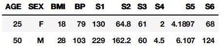
For this lab we will use the diabetes dataset.
In [ ]:
import torch

from torch import nn

from sklearn import model_selection import pandas as pd

import matplotlib.pyplot as plt import seaborn as sn

from IPython import display


import typing

%matplotlib inline
In [ ]:
diabetes_db = pd.read_csv('https://www4.stat.ncsu.edu/~boos/var.select/diabetes.tab.txt', sep='\t', header=0)

sn.pairplot(diabetes_db)
In [ ]:
diabetes_db.head(10)
We first split the data into test and training sets. For consistency and to allow for meaningful comparison the same splits are maintained in the remainder of the lab.
In [ ]:
X_train, X_test, y_train, y_test = model_selection.train_test_split( diabetes_db.loc[:, diabetes_db.columns != 'Y'], diabetes_db['Y'],

test_size=0.2, random_state=42

)

x_train = torch.from_numpy(X_train.values).float() x_test = torch.from_numpy(X_test.values).float()

y_train = torch.from_numpy(y_train.values).float() y_train = y_train.reshape(-1, 1)

y_test = torch.from_numpy(y_test.values).float() y_test = y_test.reshape(-1, 1)
We can see that all the independent variables are on different scales. This can affect gradient descent, we therefore need to normalize all features to zero mean, and unit standard deviation. The normalized value zi of xi is obtained through ![]() where μ is the mean and σ is the standard deviation of X and x , μ, σ .
where μ is the mean and σ is the standard deviation of X and x , μ, σ .
∈ RD
Q1. Complete the method and normalize x_train, x_test [2 marks] 代做人工智能作业
In [ ]:
defd  norm_set(x: torch.Tensor, mu: torch.Tensor, sigma: torch.Tensor) -> torch.tensor:

### your code here

return

###your code here
1.1 Linear Regression
We will building the linear regression model in pytorch using a custom layer.
Refering back to the lecture notes, we define y = f(x) = wT x, so we need to learn weight vector w.
Q2. Fill in the forward method of the LinearRegression class. [2 marks]
In [ ]:
classLinearRegression(nn .Module):

definit (self, num features)
super () .init ()

self.weight = nn,Parameter(torch,zeros(1, num features), requires grad=False)
def forward(self, x) :
y=0

### your code here
return y
As we need to account for the bias, we add a column of ones to the x_data
In [ ]:
# add a feature for bias

x_train = torch.cat([x_train, torch.ones(x_train.shape[0], 1)], dim=1)

x_test = torch.cat([x_test, torch.ones(x_test.shape[0], 1)], dim=1)
In [ ]:
## test the custom layer

model = LinearRegression(x_train.shape[1])

prediction = model(x_train)

prediction.shape # the output should be Nx1
The next step is to calculate the cost. For this we will use the mean squared error
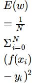
Q3. Fill in the method to calculate the squared error of for any set of labels
In [ ]:
def mean squared error(y_pred; torch.Tensor, y_true: torch.Tensor) -> torch.Tensor:
### vour code here
return
In [ ]:
cost = mean_ squared _ error(y _ train, prediction)

print(cost)
We see that using a random set of initial parameters for bias and weight, yields a relatively high error. As such, we will update the values for w using gradient descent. We will implement a custom method for gradient descent.

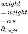
Q4. In the method below, add your code to update bias and weight using learning rate α. [2 marks]
First you need to calculate the partial derivative of the loss function with respect to the weights.
We then update the weights vector using the following equation:
In [ ]:
def gradien _descent _ step(model: nn.Module, X: torch.Tensor, y: torch.Tensor, y_pred: to

rch.Tensor,lr: float) -> None:

weight = mode1.weight

N = X.shape[0]

### your code here

# calculate the partial derivative of the loss function with respect to w 0 and w 1

#calculate the new values for bias and weight

#model.weight = nn.Parameter(weight, requires grad=False)
In [ ]: 代做人工智能作业
cost_lst = ist()

model = LinearRegression(x train.shape[1])

alpha = .1
for it in range(100):

prediction = model(x_train)

cost = mean_squared _error(y_train, prediction)

cost_lst.append(cost)

gradient descent_step (model, x _train, y _train, prediction, alpha)

fig, axs = plt.subplots(2)

axs[0].plot(list (range(it+1)), cost Ist)axs[1].scatter(prediction, y_train)

plt.show()

print (model.weight )

print('Minimum cost: [}'.format (min(cost lst)))
Q5. What conclusion if any can be drawn from the weight values? How does gender and BMI affect blood sugar levels?
What are the estimated blood sugar levels for the below examples? [2 marks] </font>
In [ ]:
### your code here
Now estimate the error on the test set. Is the error on the test set comparable to that of the train set? What can be said about the fit of the model? When does a model over/under fits?
In [ ]:
### your code here### your code here
**Q6.** Try the code with a number of learning rates that differ by orders of magnitude and record the error of the training and test sets. What do you observe on the training error? What about the error on the test set? [3 marks] 代做人工智能作业
In [ ]:
### your code here
In [ ]:
### your code here
1.2Regularized Linear Regression
In this exercise, we will be trying to create a model that fits data that is clearly not linear. We will be attempting to fit the data points seen in the graph below:
In [ ]:
x = torch.tensor([-0.99768, -0.69574, -0.40373, -0.10236, 0.22024, 0.47742, 0.82229])

y = torch.tensor([2.0885, 1.1646, 0.3287, 0.46013, 0.44808, 0.10013, -0.32952]).reshape(

-1, 1)

plt.scatter(x, y)

plt.show()
In order to fit this data we will create a new hypothesis function, which uses a fifth-order polynomial:
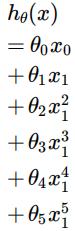
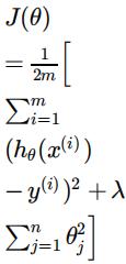
As we are fitting a small number of points with a high order model, there is a danger of overfitting. \ To attempt to avoid this we will use regularization. Our cost function becomes:
Adjust variable x to include the higher order polynomials
In [ ]:
### your code here

### hint: remember to add x_0 for the bias
Q7. Update the cost and gradient descent methods to use the regularised cost, as shown above. [4 marks] 代做人工智能作业
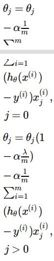
Note that the punishment for having more terms is not applied to the bias. This means that we use a different update technique for the partial derivative of θ0 , and add the regularization to all of the others:
In [ ]:
def mean_squared_error(y_true: torch.Tensor, y_pred: torch.Tensor, lam: float, theta: to
rch.tensor) -> to rch.Tensor:
### your code here
return
def gradient_descent_step(model: nn.Module, X: torch.Tensor, y: torch.Tensor, y_pred: to
rch.Tensor, lr: float) -> None:
weight = model.weight
N = X.shape[0]
your code here
###
model.weight = nn.Parameter(weight, requires_grad=False)
**Q8.** First of all, find the best value of alpha to use in order to optimize best.
Next, experiment with different values of λ and see how this affects the shape of the hypothesis. [3 marks]
In [ ]:
cost_lst = list()

model = LinearRegression(x3.shape[1]) alpha = 1 # select an appropriate alpha lam = 0 # select an appropriate lambda for it in range(100):

prediction = model(x3)

cost = mean_squared_error(y, prediction, lam, model.weight) cost_lst.append(cost)

gradient_descent_step(model, x3, y, prediction, alpha, lam) display.clear_output(wait=True)

plt.plot(list(range(it+1)), cost_lst) plt.show()

print(model.weight)

print('Minimum cost: {}'.format(min(cost_lst)))
In [ ]: 代做人工智能作业
plt.scatter(x3[:, 0], y, c='red', marker='x', label='groundtruth') outputs = model(x3)

plt.plot(x3[:, 0], outputs, c='blue', marker='o', label='prediction') plt.xlabel('x1')

plt.ylabel('y=f(x1)') plt.legend() plt.show()
更多代写:马来西亚网课代修代上 gre代考风险 代网课机构 代写Essay英文 阿德莱德(Adelaide)学术论文代写 留学生宏观经济代写
合作平台:essay代写 论文代写 写手招聘 英国留学生代写